Experiment 2
Nonlinear effect of prediction error on recognition-based episodic memory updating
Taehoon Kim, Do-Joon Yi
2022-02-22
set.seed(12345)
if (!require("magick", quietly = TRUE)) install.packages("magick")

pacman::p_load(tidyverse, knitr,
               afex, emmeans,
               psych, ggplot2, papaja, cowplot)
pacman::p_load_gh("thomasp85/patchwork", "RLesur/klippy")

options(dplyr.summarise.inform=FALSE)
options(knitr.kable.NA = '')
set_sum_contrasts() # see Singmann & Kellen (2020)

klippy::klippy()
1 Design & Procedure
f1 <- ggdraw() + draw_image("fig/F1A.png", scale = .9)
f2 <- ggdraw() + draw_image("fig/F5B.png", scale = .9)
plot_grid(f1, f2, labels = c('A', 'B'), nrow = 2, label_size = 20)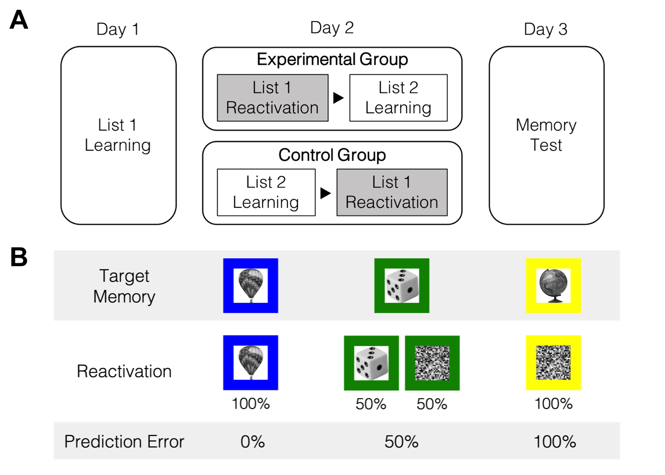
2 Day 1 & 2
첫째 날과 둘째 날에 학습한 List 1과 List 2의 물체-색상 연합학습 강도를 확인할 수 있다.
# Data
h1 <- read.csv("data/MemUdt_PE_d1t2_m.csv", header = T)
h2 <- read.csv("data/MemUdt_PE_d2t5_m.csv", header = T)
h1$List <- 'list1';
h2$List <- 'list2';
e1 <- rbind(h1, h2)

e1$SN <- factor(e1$SN)
e1$Group = factor(e1$Group, levels = c(1,2), labels=c("Experimental", "Control"))
e1$List <- factor(e1$List)
headTail(e1)
##         SN        Group Trial Block bTrial cCue IMidx      IMname    CueName
## 1        1 Experimental     1     1      1    1   147  man245.jpg  cue_1.jpg
## 2        1 Experimental     2     1      2    1    56  man092.jpg  cue_1.jpg
## 3        1 Experimental     3     1      3    1    79  man123.jpg  cue_1.jpg
## 4        1 Experimental     4     1      4    2   100  man156.jpg  cue_2.jpg
## ...   <NA>         <NA>   ...   ...    ...  ...   ...        <NA>       <NA>
## 25917   38      Control   357     4     87    1   252  man439.jpg  cue_1.jpg
## 25918   38      Control   358     4     88    1   129  man202.jpg  cue_1.jpg
## 25919   38      Control   359     4     89    2    87  man133.jpg  cue_2.jpg
## 25920   38      Control   360     4     90    3    19  man039.jpg  cue_3.jpg
##       Resp   RT Corr  List
## 1        1 0.84    1 list1
## 2        2 1.54    0 list1
## 3        1  1.6    1 list1
## 4        2  1.3    1 list1
## ...    ...  ...  ...  <NA>
## 25917    1 0.36    1 list2
## 25918    1 0.19    1 list2
## 25919    2 0.24    1 list2
## 25920    3 0.19    1 list2

table(e1$Group, e1$SN)
##
##                  1   2   3   4   5   6   7   8   9  10  11  12  13  14  15  16
##   Experimental 720   0 720   0 720   0 720 720 720   0 720   0   0   0 720   0
##   Control        0 720   0 720   0 720   0   0   0 720   0 720 720 720   0 720
##
##                 17  18  20  21  22  23  24  25  26  27  29  30  31  32  33  34
##   Experimental 720   0   0 720   0 720   0 720   0 720 720   0 720   0 720   0
##   Control        0 720 720   0 720   0 720   0 720   0   0 720   0 720   0 720
##
##                 35  36  37  38
##   Experimental 720   0 720   0
##   Control        0 720   0 720

# descriptive
e1 %>% group_by(Group, SN, List, Block) %>%
  summarise(Accuracy = mean(Corr)*100) %>%
  ungroup() %>%
  group_by(Group, List, Block) %>%
  summarise(Accuracy = mean(Accuracy)) %>%
  ungroup() %>%
  pivot_wider(names_from = 'Block', values_from = 'Accuracy') %>%
kable(digits = 4, caption = "Descriptive statistics: Group x List x Black")| Group | List | 1 | 2 | 3 | 4 |
|---|---|---|---|---|---|
| Experimental | list1 | 65.8642 | 85.7407 | 93.4568 | 98.0247 |
| Experimental | list2 | 74.8765 | 91.2346 | 96.2346 | 98.6420 |
| Control | list1 | 59.5679 | 82.5926 | 92.2840 | 97.3457 |
| Control | list2 | 67.5926 | 87.4074 | 94.9383 | 97.2222 |
e1 %>% group_by(Group, SN, List, Block) %>%
  summarise(Accuracy = mean(Corr)*100) %>%
  ungroup() %>%
  group_by(List, Block) %>%
  summarise(Accuracy = mean(Accuracy)) %>%
  ungroup() %>%
  pivot_wider(names_from = 'Block', values_from = 'Accuracy') %>%
kable(digits = 4, caption = "Descriptive statistics: List x Black")| List | 1 | 2 | 3 | 4 |
|---|---|---|---|---|
| list1 | 62.7160 | 84.1667 | 92.8704 | 97.6852 |
| list2 | 71.2346 | 89.3210 | 95.5864 | 97.9321 |
# 3way ANOVA
e1.aov <- e1 %>% group_by(Group, SN, List, Block) %>%
  summarise(Accuracy = mean(Corr)*100) %>%
  ungroup() %>%
  aov_ez(id = 'SN', dv = 'Accuracy',
         between = 'Group', within = c('List', 'Block'),
         anova_table = list(es = 'pes'))
e1.aov
## Anova Table (Type 3 tests)
##
## Response: Accuracy
## Effect df MSE F pes p.value
## 1 Group 1, 34 224.67 3.16 + .085 .084
## 2 List 1, 34 34.73 35.86 *** .513 <.001
## 3 Group:List 1, 34 34.73 0.21 .006 .652
## 4 Block 1.96, 66.56 72.24 289.63 *** .895 <.001
## 5 Group:Block 1.96, 66.56 72.24 2.73 + .074 .074
## 6 List:Block 2.17, 73.89 17.83 17.37 *** .338 <.001
## 7 Group:List:Block 2.17, 73.89 17.83 0.05 .001 .964
## ---
## Signif. codes: 0 '***' 0.001 '**' 0.01 '*' 0.05 '+' 0.1 ' ' 1
##
## Sphericity correction method: GGList 1보다 List 2의 정확도가 항상 높았지만, 그 차이는 후반부로 갈수록 감소한다.
e1.emm <- e1.aov %>%
  emmeans(pairwise ~ List | Block, type = "response") %>%
  summary(by = NULL, adjust = "bonferroni")
e1.emm[[2]]
## contrast Block estimate SE df t.ratio p.value
## list1 - list2 X1 -8.519 1.478 34 -5.765 <.0001
## list1 - list2 X2 -5.154 1.122 34 -4.592 0.0002
## list1 - list2 X3 -2.716 0.730 34 -3.719 0.0029
## list1 - list2 X4 -0.247 0.324 34 -0.762 1.0000
##
## Results are averaged over the levels of: Group
## P value adjustment: bonferroni method for 4 tests실험 1과 달리, List 1과 2의 차이는 마지막 구획에서 유의미하지 않다.
3 Day 3
# Data
e2 <- read.csv("data/MemUdt_PE_d3t6_m.csv", header = T)

e2$SN <- factor(e2$SN)
e2$Group <- factor(e2$Group, levels=c(1,2),  labels=c("Experimental","Control"))
e2$List <- factor(e2$List, levels=c(1,2,3),  labels=c("list1","list2","list3"))
e2$Cue <- factor(e2$Cue, levels=c(1,2,3,0), labels=c("cc1","cc2","cc3","lure"))
# e2$PE <- factor(e2$PE, levels=c(1,2,3,0), labels=c("pe0","pe50","pe100","lure"))
e2$CueName = factor(e2$CueName, labels=c("c0","c1","c2","c3"))
e2$Resp <- factor(e2$Resp, levels=c(1,2,3), labels=c("list1", "list2", "list3"))

e2$PE[e2$PE==0] <- NA
e2$PE[e2$PE==1] <- 0
e2$PE[e2$PE==2] <- 50
e2$PE[e2$PE==3] <- 100
str(e2)
## 'data.frame':    9720 obs. of  19 variables:
##  $ SN     : Factor w/ 36 levels "1","2","3","4",..: 1 1 1 1 1 1 1 1 1 1 ...
##  $ Group  : Factor w/ 2 levels "Experimental",..: 1 1 1 1 1 1 1 1 1 1 ...
##  $ Trial  : int  1 2 3 4 5 6 7 8 9 10 ...
##  $ List   : Factor w/ 3 levels "list1","list2",..: 3 1 1 2 1 3 1 1 1 2 ...
##  $ Cue    : Factor w/ 4 levels "cc1","cc2","cc3",..: 4 2 2 2 2 4 3 3 2 3 ...
##  $ PE     : num  NA 50 50 50 50 NA 0 0 50 0 ...
##  $ IMidx  : int  72 38 87 95 129 240 65 71 253 201 ...
##  $ IMname : chr  " man114.jpg" " man066.jpg" " man133.jpg" " man145.jpg" ...
##  $ CueName: Factor w/ 4 levels "c0","c1","c2",..: 1 3 3 3 3 1 4 4 3 4 ...
##  $ Resp   : Factor w/ 3 levels "list1","list2",..: 3 1 1 2 1 3 2 2 2 2 ...
##  $ RT     : num  2.81 3.62 5.18 1.61 1.42 ...
##  $ Corr   : int  1 1 1 1 1 1 2 2 2 1 ...
##  $ Conf   : int  4 4 4 4 4 4 4 4 4 3 ...
##  $ cRT    : num  2.487 1.26 0.876 0.981 0.891 ...
##  $ aResp  : int  7 2 2 2 2 7 3 1 2 3 ...
##  $ aRT    : num  0 4.19 0.671 0.927 0.544 ...
##  $ aCorr  : int  7 1 1 1 1 7 1 0 1 1 ...
##  $ aConf  : int  7 4 4 4 4 7 4 4 4 4 ...
##  $ aCRT   : num  0 1.604 1.74 0.803 0.463 ...
마지막 날(Day 3)에 실시한 출처기억 검사 결과를 정리하였다.
3.1 Descriptive Stats
3.1.1 List 1 & List 2
# recognition: except List 3
e2old <- e2 %>%
  filter(List == "list1" | List == "list2") %>%
  select(SN, Group, List, Cue, PE, Resp, Corr, Conf) %>%
  droplevels()

unique(e2old$List)
## [1] list1 list2
## Levels: list1 list2
unique(e2old$Resp)
## [1] list1 list2 list3
## Levels: list1 list2 list3
unique(e2old$Corr)
## [1] 1 2 3 0

e2old$Miss <- as.numeric(e2old$Corr==0) # recognition: miss rate
e2old$Correct <- as.numeric(e2old$Corr==1) # correct source memory
e2old$L1toL2 <- as.numeric(e2old$Corr==2) # source confusion
e2old$L2toL1 <- as.numeric(e2old$Corr==3) # source confusion + intrusion

glimpse(e2old)
## Rows: 6,480
## Columns: 12
## $ SN      <fct> 1, 1, 1, 1, 1, 1, 1, 1, 1, 1, 1, 1, 1, 1, 1, 1, 1, 1, 1, 1, 1,…
## $ Group   <fct> Experimental, Experimental, Experimental, Experimental, Experi…
## $ List    <fct> list1, list1, list2, list1, list1, list1, list1, list2, list2,…
## $ Cue     <fct> cc2, cc2, cc2, cc2, cc3, cc3, cc2, cc3, cc2, cc2, cc1, cc1, cc…
## $ PE      <dbl> 50, 50, 50, 50, 0, 0, 50, 0, 50, 50, 100, 100, 100, 100, 100, …
## $ Resp    <fct> list1, list1, list2, list1, list2, list2, list2, list2, list2,…
## $ Corr    <int> 1, 1, 1, 1, 2, 2, 2, 1, 1, 1, 1, 1, 3, 3, 1, 1, 1, 1, 3, 3, 1,…
## $ Conf    <int> 4, 4, 4, 4, 4, 4, 4, 3, 4, 4, 4, 3, 4, 3, 4, 4, 4, 3, 3, 3, 4,…
## $ Miss    <dbl> 0, 0, 0, 0, 0, 0, 0, 0, 0, 0, 0, 0, 0, 0, 0, 0, 0, 0, 0, 0, 0,…
## $ Correct <dbl> 1, 1, 1, 1, 0, 0, 0, 1, 1, 1, 1, 1, 0, 0, 1, 1, 1, 1, 0, 0, 1,…
## $ L1toL2  <dbl> 0, 0, 0, 0, 1, 1, 1, 0, 0, 0, 0, 0, 0, 0, 0, 0, 0, 0, 0, 0, 0,…
## $ L2toL1  <dbl> 0, 0, 0, 0, 0, 0, 0, 0, 0, 0, 0, 0, 1, 1, 0, 0, 0, 0, 1, 1, 0,…

e2oldslong <- e2old %>%
  group_by(Group, SN, List) %>%
  summarise(Correct = mean(Correct)*100,
            Miss = mean(Miss)*100,
            L1toL2 = mean(L1toL2)*100,
            L2toL1 = mean(L2toL1)*100) %>%
  ungroup() %>%
  mutate(AttrError = L1toL2 + L2toL1) %>%
  select(Group, SN, List, Correct, Miss, AttrError)

e2oldslong %>% group_by(Group, List) %>%
  summarise(Correct = mean(Correct),
            Miss = mean(Miss),
            AttrError = mean(AttrError)) %>%
  ungroup() %>%
kable(digits = 4, caption = "Descriptive statistics: Group x List")| Group | List | Correct | Miss | AttrError |
|---|---|---|---|---|
| Experimental | list1 | 75.4321 | 3.2716 | 21.2963 |
| Experimental | list2 | 66.0494 | 2.2222 | 31.7284 |
| Control | list1 | 71.4198 | 4.6296 | 23.9506 |
| Control | list2 | 70.6790 | 3.5802 | 25.7407 |
3.1.2 List 3
e2new <- e2 %>%
  filter(List == "list3") %>%
  select(SN, Group, Resp, Corr, Conf) %>%
  droplevels()
head(e2new)
##   SN        Group  Resp Corr Conf
## 1  1 Experimental list3    1    4
## 2  1 Experimental list3    1    4
## 3  1 Experimental list3    1    4
## 4  1 Experimental list3    1    4
## 5  1 Experimental list3    1    4
## 6  1 Experimental list3    1    2
unique(e2new$Resp)
## [1] list3 list1 list2
## Levels: list1 list2 list3
unique(e2new$Corr)
## [1] 1 0

e2new %>% group_by(Group, SN) %>%
  summarise(FA = 100 - mean(Corr)*100) %>%
  ungroup() %>%
  group_by(Group) %>%
  summarise(FA = mean(FA)) %>%
  ungroup() %>%
kable(digits = 4, caption = "Descriptive statistics: Group")| Group | FA |
|---|---|
| Experimental | 2.7160 |
| Control | 4.3827 |
3.2 Miss
e2oldslong %>% aov_ez(id = 'SN', dv = 'Miss',
                      between = 'Group', within = 'List',
                      anova_table = list(es = 'pes'))
## Anova Table (Type 3 tests)
##
## Response: Miss
## Effect df MSE F pes p.value
## 1 Group 1, 34 13.13 2.53 .069 .121
## 2 List 1, 34 6.93 2.86 .078 .100
## 3 Group:List 1, 34 6.93 0.00 <.001 >.999
## ---
## Signif. codes: 0 '***' 0.001 '**' 0.01 '*' 0.05 '+' 0.1 ' ' 1List 1과 List 2의 항목을 “본 적 없다”고 답하는 비율은 매우 낮았고, 조건간 차이도 유의미하지 않았다.
3.3 False alarm
e2new %>% group_by(Group, SN) %>%
  summarise(FA = 100 - mean(Corr)*100) %>%
  ungroup() %>%
  aov_ez(id = 'SN', dv = 'FA', between = 'Group',
         anova_table = list(es = 'pes'))
## Anova Table (Type 3 tests)
##
## Response: FA
## Effect df MSE F pes p.value
## 1 Group 1, 34 30.26 0.83 .024 .370
## ---
## Signif. codes: 0 '***' 0.001 '**' 0.01 '*' 0.05 '+' 0.1 ' ' 1List 3의 항목을 “봤다”고 답한 비율도 낮았다. 집단 차이는 유의미하지 않았다.
3.4 Source accuracy
e2oldslong %>% aov_ez(id = 'SN', dv = 'Correct',
                      between = 'Group', within = 'List',
                      anova_table = list(es = 'pes'))
## Anova Table (Type 3 tests)
##
## Response: Correct
## Effect df MSE F pes p.value
## 1 Group 1, 34 118.77 0.01 <.001 .905
## 2 List 1, 34 109.56 4.21 * .110 .048
## 3 Group:List 1, 34 109.56 3.07 + .083 .089
## ---
## Signif. codes: 0 '***' 0.001 '**' 0.01 '*' 0.05 '+' 0.1 ' ' 13.4.0.1 Source misattribution
e2AttrErr.aov <- e2oldslong %>%
  aov_ez(id = 'SN', dv = 'AttrError',
         between = 'Group', within = 'List',
         anova_table = list(es = 'pes'))
e2AttrErr.aov
## Anova Table (Type 3 tests)
##
## Response: AttrError
## Effect df MSE F pes p.value
## 1 Group 1, 34 81.07 0.62 .018 .438
## 2 List 1, 34 102.44 6.56 * .162 .015
## 3 Group:List 1, 34 102.44 3.28 + .088 .079
## ---
## Signif. codes: 0 '***' 0.001 '**' 0.01 '*' 0.05 '+' 0.1 ' ' 1# custom contrast
e2AttrErr.emm <- e2AttrErr.aov %>% emmeans(~ List*Group)
con <- emmeans:::trt.vs.ctrl.emmc(1:4)
ExpL2L1 <- c(-1, 1,0,0)
ConL2L1 <- c(0,0,-1, 1)
L2ExpCon <- c(0,1,0,-1)
con <- data.frame(ExpL2L1, ConL2L1, L2ExpCon)
contrast(e2AttrErr.emm, con, adjust = "bonferroni")## contrast estimate SE df t.ratio p.value
## ExpL2L1 10.43 3.37 34 3.092 0.0119
## ConL2L1 1.79 3.37 34 0.531 1.0000
## L2ExpCon 5.99 3.49 34 1.716 0.2860
##
## P value adjustment: bonferroni method for 3 testsANOVA에서 List 2를 List 1으로 오기억하는 경우가 반대보다 높았으나, 집단 차이는 유의미하지 않았다. 그러나 사후비교에서 실험집단의 경우에만 List 2 오귀인이 List 1 오귀인보다 높았다(비대칭적 오귀인 분포).
3.5 Prediction error effects
e2PEslong <- e2old %>%
  filter(List == 'list2') %>%
  group_by(Group, SN, PE) %>%
  droplevels() %>%
  summarise(L2toL1 = mean(L2toL1)) %>%
  ungroup()

str(e2PEslong)
## tibble [108 × 4] (S3: tbl_df/tbl/data.frame)
##  $ Group : Factor w/ 2 levels "Experimental",..: 1 1 1 1 1 1 1 1 1 1 ...
##  $ SN    : Factor w/ 36 levels "1","2","3","4",..: 1 1 1 3 3 3 5 5 5 7 ...
##  $ PE    : num [1:108] 0 50 100 0 50 100 0 50 100 0 ...
##  $ L2toL1: num [1:108] 0.2 0.3 0.533 0.167 0.233 ...
e2PEslong %>%
group_by(Group, PE) %>%
summarise(L2toL1 = mean(L2toL1)) %>%
ungroup() %>%
pivot_wider(names_from = 'PE', values_from = 'L2toL1') %>%
kable(digits = 4, caption = "Descriptive statistics: Group x PE")| Group | 0 | 50 | 100 |
|---|---|---|---|
| Experimental | 0.2667 | 0.3648 | 0.3204 |
| Control | 0.2519 | 0.2426 | 0.2778 |
e2PE.aov <- e2PEslong %>%
  aov_ez(id = 'SN', dv = 'L2toL1',
         between = 'Group', within = 'PE',
         anova_table = list(es = 'pes'))
e2PE.aov
## Anova Table (Type 3 tests)
##
## Response: L2toL1
## Effect df MSE F pes p.value
## 1 Group 1, 34 0.03 2.94 + .080 .095
## 2 PE 1.98, 67.46 0.01 2.87 + .078 .064
## 3 Group:PE 1.98, 67.46 0.01 3.73 * .099 .029
## ---
## Signif. codes: 0 '***' 0.001 '**' 0.01 '*' 0.05 '+' 0.1 ' ' 1
##
## Sphericity correction method: GG집단과 예측오류 수준의 상호작용이 유의미하였다.
# custom contrast
e2PE.emm <- e2PE.aov %>% emmeans(~ Group*PE)
Exp0to50 <- c(-1,0,1,0,0,0)
Exp0to100 <- c(-1,0,0,0,1,0)
Exp100to50 <- c(0,0,1,0,-1,0)
Con0to50 <- c(0,-1,0,1,0,0)
Con0to100 <- c(0,-1,0,0,0,1)
Con100to50 <- c(0,0,0,1,0,-1)
ExpCon50 <- c(0,0,1,-1,0,0)
con <- data.frame(Exp0to50, Exp0to100, Exp100to50,
                  Con0to50, Con0to100, Con100to50, ExpCon50)
contrast(e2PE.emm, con, adjust = "Bonferroni")
## contrast estimate SE df t.ratio p.value
## Exp0to50 0.09815 0.0287 34 3.424 0.0114
## Exp0to100 0.05370 0.0301 34 1.787 0.5799
## Exp100to50 0.04444 0.0278 34 1.596 0.8377
## Con0to50 -0.00926 0.0287 34 -0.323 1.0000
## Con0to100 0.02593 0.0301 34 0.863 1.0000
## Con100to50 -0.03519 0.0278 34 -1.264 1.0000
## ExpCon50 0.12222 0.0412 34 2.969 0.0381
##
## P value adjustment: bonferroni method for 7 tests실험집단에서만 PE50의 침범반응이 PE0보다 컸다.
emm.t2 <- e2PE.aov %>% emmeans(pairwise ~ PE | Group)
emm.t2[[1]] %>% contrast("poly") %>%
    summary(by = NULL, adjust = "Bonferroni")
## contrast Group estimate SE df t.ratio p.value
## linear Experimental 0.0537 0.0301 34 1.787 0.3313
## quadratic Experimental -0.1426 0.0479 34 -2.979 0.0212
## linear Control 0.0259 0.0301 34 0.863 1.0000
## quadratic Control 0.0444 0.0479 34 0.929 1.0000
##
## P value adjustment: bonferroni method for 4 testsemm.t2[[1]] %>% contrast(interaction = c("poly", "consec"),
by = NULL, adjust = "Bonferroni")## PE_poly Group_consec estimate SE df t.ratio p.value
## linear Control - Experimental -0.0278 0.0425 34 -0.654 1.0000
## quadratic Control - Experimental 0.1870 0.0677 34 2.763 0.0183
##
## P value adjustment: bonferroni method for 2 tests이차함수 추세(quadratic trend)에서 PE와 집단의 상호작용이 유의미하였다(가정 중요한 결과).
3.6 Source confidence
e2old %>% filter(Corr == 2 | Corr == 3) %>%
  droplevels() %>%
  group_by(Group, SN, List) %>%
  summarise(Confid = mean(Conf)) %>%
  ungroup() %>%
  group_by(Group, List) %>%
  summarise(Confid = mean(Confid)) %>%
  ungroup() %>%
  pivot_wider(names_from = 'List', values_from = 'Confid') %>%
kable(digits = 4, caption = "Descriptive statistics: Group x List")| Group | list1 | list2 |
|---|---|---|
| Experimental | 2.7256 | 3.0859 |
| Control | 2.7576 | 3.0635 |
e2old %>% filter(Corr == 2 | Corr == 3) %>%
  droplevels() %>%
  group_by(Group, SN, List) %>%
  summarise(Confid = mean(Conf)) %>%
  ungroup() %>%
  aov_ez(id = 'SN', dv = 'Confid',
         between = 'Group', within = 'List',
         anova_table = list(es = 'pes'))
## Anova Table (Type 3 tests)
##
## Response: Confid
## Effect df MSE F pes p.value
## 1 Group 1, 34 0.42 0.00 <.001 .975
## 2 List 1, 34 0.06 32.43 *** .488 <.001
## 3 Group:List 1, 34 0.06 0.22 .006 .644
## ---
## Signif. codes: 0 '***' 0.001 '**' 0.01 '*' 0.05 '+' 0.1 ' ' 1List 1보다 List 2에 대한 확신도가 더 높았다.
# List 2 misattr X PE: Confidence
e2old %>% filter(List == 'list2') %>%
  droplevels() %>%
  group_by(Group, SN, PE) %>%
  summarise(Conf = mean(Conf)) %>%
  ungroup() %>%
  group_by(Group, PE) %>%
  summarise(Conf = mean(Conf)) %>%
  ungroup() %>%
  pivot_wider(names_from = 'PE', values_from = 'Conf') %>%
kable(digits = 4, caption = "Descriptive statistics: Group x PE")| Group | 0 | 50 | 100 |
|---|---|---|---|
| Experimental | 3.1222 | 3.1981 | 3.1630 |
| Control | 3.1426 | 3.1667 | 3.1278 |
e2old %>% filter(List == 'list2') %>%
  droplevels() %>%
  group_by(Group, SN, PE) %>%
  summarise(Conf = mean(Conf)) %>%
  ungroup() %>%
  aov_ez(id = 'SN', dv = 'Conf',
         between = 'Group', within = 'PE',
         anova_table = list(es = 'pes'))
## Anova Table (Type 3 tests)
##
## Response: Conf
## Effect df MSE F pes p.value
## 1 Group 1, 34 0.61 0.01 <.001 .919
## 2 PE 1.93, 65.62 0.03 0.83 .024 .435
## 3 Group:PE 1.93, 65.62 0.03 0.30 .009 .735
## ---
## Signif. codes: 0 '***' 0.001 '**' 0.01 '*' 0.05 '+' 0.1 ' ' 1
##
## Sphericity correction method: GG3.7 Associative Memory
3.7.1 Accuracy
e2 %>% filter(List != "list3", Resp != "list3") %>%
  group_by(Group, SN, List) %>%
  summarise(Accuracy = mean(aCorr)*100) %>%
  ungroup() %>%
  group_by(Group, List) %>%
  summarise(Accuracy = mean(Accuracy)) %>%
  ungroup() %>%
  pivot_wider(names_from = 'List', values_from = 'Accuracy') %>%
kable(digits = 4, caption = "Descriptive statistics: Group x List")| Group | list1 | list2 |
|---|---|---|
| Experimental | 86.1648 | 89.9063 |
| Control | 85.2086 | 87.4866 |
e2 %>% filter(List != "list3", Resp != "list3") %>%
  group_by(Group, SN, List) %>%
  summarise(Accuracy = mean(aCorr)*100) %>%
  ungroup() %>%
  aov_ez(id = 'SN', dv = 'Accuracy',
         between = 'Group', within = 'List',
         anova_table = list(es = 'pes'))
## Anova Table (Type 3 tests)
##
## Response: Accuracy
## Effect df MSE F pes p.value
## 1 Group 1, 34 107.50 0.48 .014 .494
## 2 List 1, 34 18.78 8.68 ** .203 .006
## 3 Group:List 1, 34 18.78 0.51 .015 .479
## ---
## Signif. codes: 0 '***' 0.001 '**' 0.01 '*' 0.05 '+' 0.1 ' ' 13.7.2 Confidence
e2 %>% filter(List != "list3", Resp != "list3") %>%
  group_by(Group, SN, List) %>%
  summarise(Confident = mean(aConf)) %>%
  ungroup() %>%
  group_by(Group, List) %>%
  summarise(Confident = mean(Confident)) %>%
  ungroup() %>%
  pivot_wider(names_from = 'List', values_from = 'Confident') %>%
kable(digits = 4, caption = "Descriptive statistics: Group x List")| Group | list1 | list2 |
|---|---|---|
| Experimental | 3.5065 | 3.5713 |
| Control | 3.4765 | 3.5287 |
e2 %>% filter(List != "list3", Resp != "list3") %>%
  group_by(Group, SN, List) %>%
  summarise(Confident = mean(aConf)) %>%
  ungroup() %>%
  aov_ez(id = 'SN', dv = 'Confident',
         between = 'Group', within = 'List',
         anova_table = list(es = 'pes'))
## Anova Table (Type 3 tests)
##
## Response: Confident
## Effect df MSE F pes p.value
## 1 Group 1, 34 0.24 0.10 .003 .753
## 2 List 1, 34 0.02 2.68 .073 .111
## 3 Group:List 1, 34 0.02 0.03 <.001 .861
## ---
## Signif. codes: 0 '***' 0.001 '**' 0.01 '*' 0.05 '+' 0.1 ' ' 14 Plots
e2cnt <- e2old %>%
  group_by(Group, SN, List, Resp) %>%
  summarise(n = n()) %>%
  mutate(prop = n/sum(n)) %>%
  ungroup() %>%
  filter(Resp != 'list3') %>%
  droplevels()
# print(e2cnt, n=20)

tmp0 <- e2cnt %>%
  group_by(Group, List, Resp) %>%
  summarise(MN = mean(prop),
            SD = sd(prop)) %>%
  ungroup()

tmp1 <- e2cnt %>%
  filter(Group == 'Experimental') %>%
  droplevels() %>%
  papaja::wsci(id = 'SN',
               factor = c('List', 'Resp'),
               dv = 'prop') %>%
  mutate(Group = "Experimental") %>%
  rename("wsci" = "prop")

tmp2 <- e2cnt %>%
  filter(Group == 'Control') %>%
  droplevels() %>%
  papaja::wsci(id = 'SN',
               factor = c('List', 'Resp'),
               dv = 'prop') %>%
  mutate(Group = "Control") %>%
  rename("wsci" = "prop")

tmp3 <- merge(tmp1, tmp2, all = TRUE)

e2cnt.g <- merge(tmp0, tmp3, by = c("Group", "List", "Resp"), all = TRUE)


F3A <- ggplot(data=e2cnt.g, aes(x=List, y=MN, fill=Resp)) +
  geom_bar(stat='identity', width=0.7, color="black",
           position=position_dodge(.8)) +
  geom_errorbar(aes(x=List, ymin=MN-wsci, ymax=MN+wsci, group=Resp),
                position = position_dodge(0.8), width=0.3,
                show.legend = FALSE) +
  facet_grid(.~Group) +
  scale_x_discrete(labels=c("List 1","List 2")) +
  scale_y_continuous(breaks=c(0, .2, .4, .6, .8, 1)) +
  scale_fill_manual(values = c("#feb24c", "#91bfdb"),
                    labels = c("Day 1", "Day 2")) +
  labs(x = "Object List", y = "Proportion", fill='Response') +
  coord_cartesian(ylim = c(0, 1), clip = "on") +
  theme_bw(base_size = 18) +
  theme(panel.grid.major = element_blank(),
        panel.grid.minor = element_blank())
F3A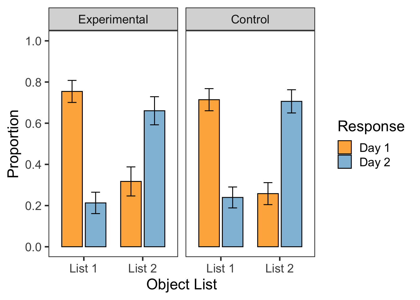
tmp0 <- e2PEslong %>%
  group_by(Group, PE) %>%
  summarise(MN = mean(L2toL1)) %>%
  ungroup()

tmp1 <- e2PEslong %>%
  filter(Group == 'Experimental') %>%
  droplevels() %>%
  papaja::wsci(id = 'SN',
               factor = 'PE',
               dv = 'L2toL1') %>%
  mutate(Group = "Experimental") %>%
  rename("wsci" = "L2toL1")

tmp2 <- e2PEslong %>%
  filter(Group == 'Control') %>%
  droplevels() %>%
  papaja::wsci(id = 'SN',
               factor = 'PE',
               dv = 'L2toL1') %>%
  mutate(Group = "Control") %>%
  rename("wsci" = "L2toL1")

tmp3 <- merge(tmp1, tmp2, all = TRUE)

e2PEg <- merge(tmp0, tmp3, by = c("Group", "PE"), all = TRUE)


F3B <- ggplot(data=e2PEg, aes(x=PE, y=MN, group=Group,
                              ymin=MN-wsci, ymax=MN+wsci)) +
  geom_line(position = position_dodge(width=10)) +
  geom_errorbar(position = position_dodge(10), width=5,
                show.legend = FALSE) +
  geom_point(aes(shape=Group, fill=Group),
             size=4, color='black', stroke=1,
             position=position_dodge(width=10)) +
  scale_x_continuous(breaks=c(0, 50, 100)) +
  scale_y_continuous(breaks=c(0, .1, .2, .3, .4, .5)) +
  scale_shape_manual(values = c(21, 23)) +
  scale_fill_manual(values = c("black", "white")) +
  labs(x = "Prediction Error (%)", y = "Proportion Intrusion", fill='Group') +
  coord_cartesian(ylim = c(0, 0.5), clip = "on") +
  theme_bw(base_size = 18) +
  theme(panel.grid.major = element_blank(),
        panel.grid.minor = element_blank(),
        aspect.ratio = 1)
F3B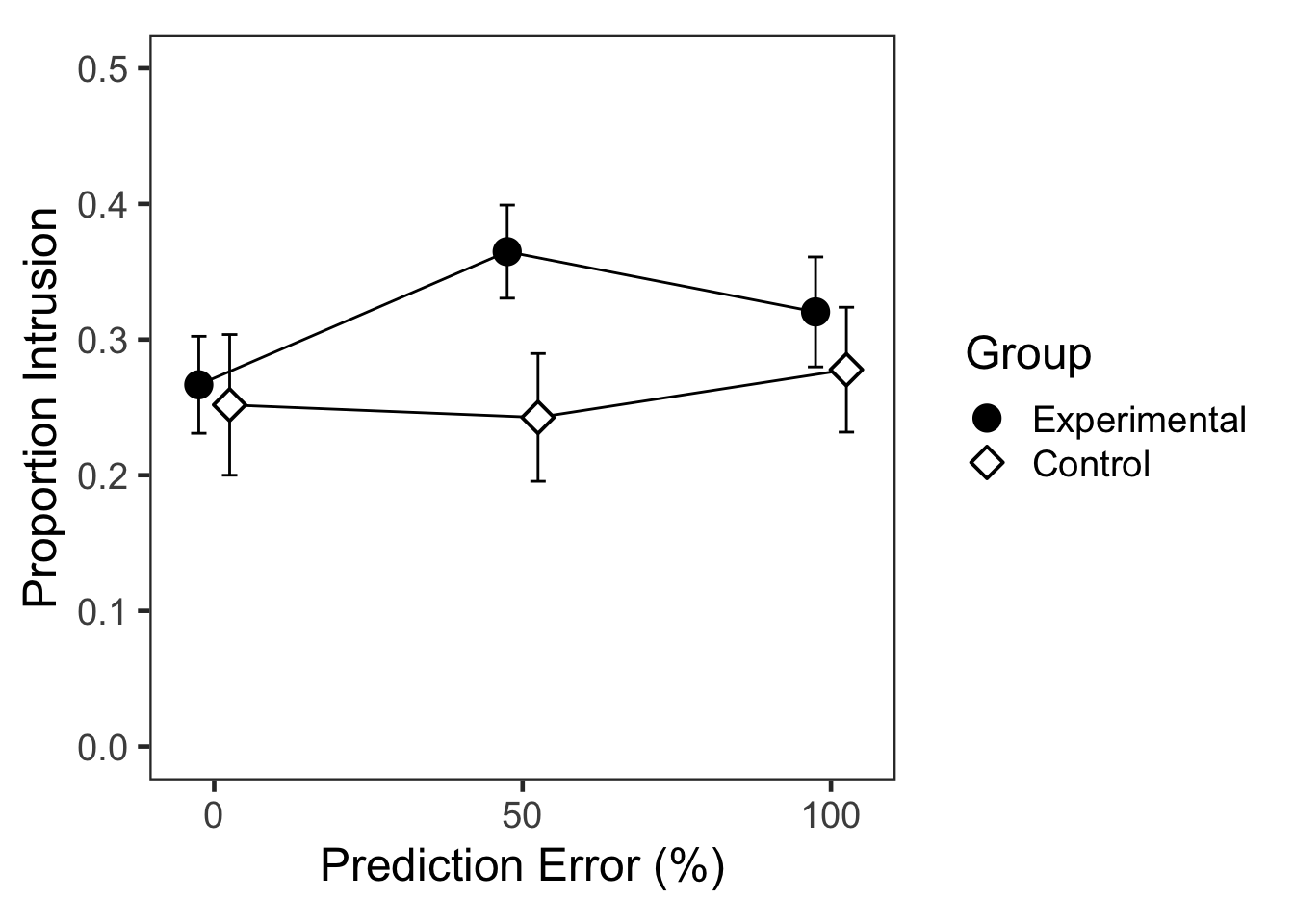
# all plots
# cowplot::plot_grid(F2A, F3A, ncol = 1, labels = c('A', 'B'), label_size = 20)
# cowplot::plot_grid(F2B, F3B, ncol = 1, labels = c('A', 'B'), label_size = 20)


# https://www.datanovia.com/en/blog/how-to-add-p-values-to-ggplot-facets/
5 Session Info
sessionInfo()
## R version 4.1.2 (2021-11-01)
## Platform: x86_64-apple-darwin17.0 (64-bit)
## Running under: macOS Monterey 12.2.1
##
## Matrix products: default
## LAPACK: /Library/Frameworks/R.framework/Versions/4.1/Resources/lib/libRlapack.dylib
##
## locale:
## [1] en_US.UTF-8/en_US.UTF-8/en_US.UTF-8/C/en_US.UTF-8/en_US.UTF-8
##
## attached base packages:
## [1] stats     graphics  grDevices utils     datasets  methods   base
##
## other attached packages:
##  [1] klippy_0.0.0.9500 patchwork_1.1.1   cowplot_1.1.1     papaja_0.1.0.9997
##  [5] psych_2.1.9       emmeans_1.7.2     afex_1.0-1        lme4_1.1-28
##  [9] Matrix_1.4-0      knitr_1.37        forcats_0.5.1     stringr_1.4.0
## [13] dplyr_1.0.8       purrr_0.3.4       readr_2.1.2       tidyr_1.2.0
## [17] tibble_3.1.6      ggplot2_3.3.5     tidyverse_1.3.1   magick_2.7.3
## [21] icons_0.2.0
##
## loaded via a namespace (and not attached):
##   [1] TH.data_1.1-0       minqa_1.2.4         colorspace_2.0-3
##   [4] ellipsis_0.3.2      rsconnect_0.8.25    rprojroot_2.0.2
##   [7] estimability_1.3    fs_1.5.2            rstudioapi_0.13
##  [10] farver_2.1.0        remotes_2.4.2       fansi_1.0.2
##  [13] mvtnorm_1.1-3       lubridate_1.8.0     xml2_1.3.3
##  [16] codetools_0.2-18    splines_4.1.2       mnormt_2.0.2
##  [19] cachem_1.0.6        pkgload_1.2.4       jsonlite_1.7.3
##  [22] nloptr_2.0.0        broom_0.7.12        dbplyr_2.1.1
##  [25] compiler_4.1.2      httr_1.4.2          backports_1.4.1
##  [28] assertthat_0.2.1    fastmap_1.1.0       cli_3.2.0
##  [31] htmltools_0.5.2     prettyunits_1.1.1   tools_4.1.2
##  [34] lmerTest_3.1-3      coda_0.19-4         gtable_0.3.0
##  [37] glue_1.6.1          reshape2_1.4.4      rappdirs_0.3.3
##  [40] Rcpp_1.0.8          carData_3.0-5       cellranger_1.1.0
##  [43] jquerylib_0.1.4     vctrs_0.3.8         nlme_3.1-155
##  [46] xfun_0.29           ps_1.6.0            brio_1.1.3
##  [49] testthat_3.1.2      rvest_1.0.2         lifecycle_1.0.1
##  [52] pacman_0.5.1        devtools_2.4.3      MASS_7.3-55
##  [55] zoo_1.8-9           scales_1.1.1        hms_1.1.1
##  [58] parallel_4.1.2      sandwich_3.0-1      yaml_2.3.5
##  [61] curl_4.3.2          memoise_2.0.1       sass_0.4.0
##  [64] stringi_1.7.6       highr_0.9           desc_1.4.0
##  [67] boot_1.3-28         pkgbuild_1.3.1      rlang_1.0.1
##  [70] pkgconfig_2.0.3     evaluate_0.15       lattice_0.20-45
##  [73] labeling_0.4.2      processx_3.5.2      tidyselect_1.1.2
##  [76] plyr_1.8.6          magrittr_2.0.2      R6_2.5.1
##  [79] generics_0.1.2      multcomp_1.4-18     DBI_1.1.2
##  [82] pillar_1.7.0        haven_2.4.3         withr_2.4.3
##  [85] survival_3.2-13     abind_1.4-5         modelr_0.1.8
##  [88] crayon_1.5.0        car_3.0-12          utf8_1.2.2
##  [91] tmvnsim_1.0-2       tzdb_0.2.0          rmarkdown_2.11
##  [94] usethis_2.1.5       grid_4.1.2          readxl_1.3.1
##  [97] callr_3.7.0         reprex_2.0.1        digest_0.6.29
## [100] xtable_1.8-4        numDeriv_2016.8-1.1 munsell_0.5.0
## [103] bslib_0.3.1         sessioninfo_1.2.2
Copyright © 2022 CogNIPS. All rights reserved.