Experiment 1
Self-Priority Effects on Nonspatial Working Memory
Woojeong Lee & Do-Joon Yi
2025-10-01
pacman::p_load(tidyverse, psych, knitr, rstatix, BayesFactor, Superpower)
pacman::p_load(ggpubr, see, cowplot)
pacman::p_load_gh("thomasp85/patchwork", "rlesur/klippy")
if (!requireNamespace("Rmisc", quietly = TRUE)) install.packages("Rmisc") # never load directly

set.seed(1234567) # for reproducibility
options(dplyr.summarise.inform=FALSE) # suppress warning in regards to regrouping
options(knitr.kable.NA = '')
options("scipen" = 100) # https://rfriend.tistory.com/224
nIter <- 1e6 # Monte Carlo simulations for error < 1%. default = 1e4
tOff <- 2.5 # RTtrimming
klippy::klippy()
# Excluding Ss
rm_subject <- function(df, rx){
  for (i in rx){
    df <- df %>% filter(SN != i) %>% droplevels()
  }
  cat(sprintf('%d removed & %d left',
              length(unique(rx)),
              length(unique(df$SN))))
  return(df)
}

# Plot for outlier check
# stat summary plot to 25% quartile and 75% quartile
# https://bit.ly/3iFpV07
single_raincloud_plot <- function(df, Y, xMin, xMax, xBy, xLab){
  df %>% ggplot(aes(x = 1, y = Y)) +
    geom_violinhalf(flip = c(1,3), width = 0.5, color = "grey70", fill = "gray70") +
    geom_point(aes(0.8, Y), size = 1.5,
               color = "grey50", fill = "grey50", alpha = .5,
               position = position_jitter(width = 0.15, height = 0)) +
    geom_boxplot(width=0.05, alpha = 0.5, outliers = FALSE) +
    scale_y_continuous(breaks=seq(xMin,xMax,by=xBy)) +
    coord_flip(ylim = c(xMin, xMax), clip = "on") +
    labs(y = xLab) +
    theme_bw(base_size = 18) +
    theme(panel.grid.major = element_blank(),
          panel.grid.minor = element_blank(),
          axis.title.y = element_blank(),
          axis.ticks.y = element_blank(),
          axis.text.y = element_blank(),
          aspect.ratio = .3)
}

# rgb(220, 50, 32, maxColorValue = 255) # red = #DC3220
# rgb(0, 90, 181, maxColorValue = 255) # blue = #005AB5

# Plot for results
plotMatchLabel <- function(df, ylabel, ymin, ymax, yby,
                           OminusS, ymin2, ymax2, yby2) {
  names(df)[ncol(df)] <- "DV" # assuming DV on the last column

  df.g <- df %>%
    Rmisc::summarySEwithin(measurevar = 'DV', idvar = 'SN',
                           withinvars = c("Matching", "Label"))

  df.w <- df %>%
    unite("temp", c("Matching", "Label")) %>%
    pivot_wider(id_cols = SN, names_from = temp, values_from = DV)

  doff <- 0.03
  tmp <- runif(nrow(df.w), -doff, doff)
  spd1 <- rep(-0.14,nrow(df.w)) + tmp
  spd2 <- rep( 0.14,nrow(df.w)) + tmp

  F1 <- ggplot() +
    geom_bar(data=df.g, aes(x = Matching, y = DV, fill = Label), alpha = .6,
             stat="identity", width=0.7, linewidth=0.5, color="black",
             position=position_dodge(.8)) +
    scale_fill_manual(values=c('#DC3220', '#005AB5'),
                      labels=c("Self", "Stranger")) +
    geom_segment(data=df.w, color="black", alpha = 0.3,
                 aes(x=1+spd1, y=Match_Self, xend=1+spd2, yend=Match_Stranger)) +
    geom_segment(data=df.w, color="black", alpha = 0.3,
                 aes(x=2+spd1, y=Nonmatch_Self, xend=2+spd2, yend=Nonmatch_Stranger)) +
    geom_linerange(data=df.g, aes(x=Matching, ymin=DV-ci, ymax=DV+ci, group=Label),
                   linewidth=1, position=position_dodge(0.8)) +
    labs(x = "Matching", y = ylabel, fill='Label ') +
    coord_cartesian(ylim = c(ymin, ymax), clip = "on") +
    scale_y_continuous(breaks=seq(ymin, ymax, by = yby)) +
    theme_bw(base_size = 18) +
    theme(legend.position="top",
          legend.spacing.x = unit(0.5, 'lines'),
          legend.margin = margin(0, 0, 0, 0),
          legend.background = element_blank(),
          panel.grid.major = element_blank(),
          panel.grid.minor = element_blank())

  if (OminusS) { # Boolean: Stranger - Self
    df2.w <- df.w %>%
      mutate(Match = Match_Stranger - Match_Self,
             Nonmatch = Nonmatch_Stranger - Nonmatch_Self) %>%
      select(SN, Match, Nonmatch)
  } else {
    df2.w <- df.w %>%
      mutate(Match = Match_Self - Match_Stranger,
             Nonmatch = Nonmatch_Self - Nonmatch_Stranger) %>%
      select(SN, Match, Nonmatch)
  }

  df2 <- df2.w %>%
    pivot_longer(cols = c(Match, Nonmatch), names_to = "Matching", values_to = "SPE")

  df2.g <- df2 %>%
    mutate(Matching = factor(Matching)) %>%
    Rmisc::summarySEwithin(measurevar = "SPE", withinvars = "Matching", idvar = "SN")

  moff <- 0.1
  doff <- 0.05
  vpd <- rep(c(1-moff, 2+moff), nrow(df2)/2) # violin position dodge
  dpd <- rep(c(1+moff, 2-moff), nrow(df2)/2) + # dot position dodge
    rep(runif(nrow(df2)/2, -doff, doff), each=2)

  F2 <- cbind(df2, vpd, dpd) %>%
    ggplot(aes(x = Matching, y = SPE, group = Matching)) +
    geom_pointrange(data=df2.g, aes(x = Matching, ymin = SPE-ci, ymax = SPE+ci),
                    linewidth = 1, size = 0.5, color = "black") +
    geom_point(data=df2.g, aes(x = Matching, y = SPE),
               size=3, color = "black", show.legend = FALSE) +
    geom_hline(yintercept = 0) +
    geom_violinhalf(aes(x = vpd, y = SPE, group = Matching),
                    flip = c(1,3), width = 0.7, fill = "gray70") +
    geom_line(aes(x = dpd, y = SPE, group = SN), color = "black", alpha = 0.3) +
    labs(x = "Matching",
         y = ifelse (OminusS, # Boolean: Stranger - Self
                     "Stranger - Self", "Self - Stranger")) +
    coord_cartesian(ylim = c(ymin2, ymax2), clip = "on") +
    scale_y_continuous(breaks=seq(ymin2, ymax2, by = yby2)) +
    theme_bw(base_size = 18) +
    theme(panel.grid.major = element_blank(),
          panel.grid.minor = element_blank())

  F1 + F2 + plot_layout(nrow = 1, widths = c(2, 1.2))
}

plotOrderIdentity <- function(df, ylabel, ymin, ymax, yby,
                              OminusS, ymin2, ymax2, yby2, flo = 0.1) {
  # assuming 1-4: SN, Order, Label, DV
  names(df)[ncol(df)] <- "DV" # assuming DV on the last column

  df.g <- df %>%
    Rmisc::summarySEwithin(measurevar = 'DV', idvar = 'SN',
                           withinvars = c("Order", "Identity"))

  df.w <- df %>%
    unite("temp", c("Order", "Identity")) %>%
    pivot_wider(id_cols = SN, names_from = temp, values_from = DV)

  doff <- 0.03
  tmp <- runif(nrow(df.w), -doff, doff)
  spd1 <- rep(-0.14,nrow(df.w)) + tmp
  spd2 <- rep( 0.14,nrow(df.w)) + tmp

  F1 <- ggplot() +
    geom_bar(data=df.g, aes(x = Order, y = DV, fill = Identity), alpha = .6,
             stat="identity", width=0.7, linewidth=0.5, color="black",
             position=position_dodge(.8)) +
    scale_fill_manual(values=c('#DC3220', '#005AB5'),
                      labels=c("Self", "Stranger")) +
    geom_segment(data=df.w, color="black", alpha = 0.3,
                 aes(x=1+spd1, y=First_Self, xend=1+spd2, yend=First_Stranger)) +
    geom_segment(data=df.w, color="black", alpha = 0.3,
                 aes(x=2+spd1, y=Second_Self, xend=2+spd2, yend=Second_Stranger)) +
    geom_linerange(data=df.g, aes(x=Order, ymin=DV-ci, ymax=DV+ci, group=Identity),
                   linewidth=1, position=position_dodge(0.8)) +
    labs(x = "Order", y = ylabel, fill='Identity ') +
    coord_cartesian(ylim = c(ymin, ymax), clip = "on") +
    scale_y_continuous(breaks=seq(ymin, ymax, by = yby)) +
    theme_bw(base_size = 18) +
    theme(legend.position="top",
          legend.spacing.x = unit(0.5, 'lines'),
          legend.margin = margin(0, 0, 0, 0),
          legend.background = element_blank(),
          panel.grid.major = element_blank(),
          panel.grid.minor = element_blank())

  if (OminusS) { # Boolean: Stranger - Self
    df2.w <- df.w %>%
      mutate(First = First_Stranger - First_Self,
             Second = Second_Stranger - Second_Self) %>%
      select(SN, First, Second)
  } else {
    df2.w <- df.w %>%
      mutate(First = First_Self - First_Stranger,
             Second = Second_Self - Second_Stranger) %>%
      select(SN, First, Second)
  }

  df2 <- df2.w %>%
    pivot_longer(cols = c(First, Second), names_to = "Order", values_to = "SPE")

  df2.g <- df2 %>%
    mutate(Order = factor(Order)) %>%
    Rmisc::summarySEwithin(measurevar = "SPE", withinvars = "Order", idvar = "SN")

  moff <- 0.1
  doff <- 0.05
  vpd <- rep(c(1-moff, 2+moff), nrow(df2)/2) # violin position dodge
  dpd <- rep(c(1+moff, 2-moff), nrow(df2)/2) + # dot position dodge
    rep(runif(nrow(df2)/2, -doff, doff), each=2)

  F2 <- cbind(df2, vpd, dpd) %>%
    ggplot(aes(x = Order, y = SPE, group = Order)) +
    geom_pointrange(data=df2.g, aes(x = Order, ymin = SPE-ci, ymax = SPE+ci),
                    linewidth = 1, size = 0.5, color = "black") +
    geom_point(data=df2.g, aes(x = Order, y = SPE),
               size=3, color = "black", show.legend = FALSE) +
    geom_hline(yintercept = 0) +
    geom_violinhalf(aes(x = vpd, y = SPE, group = Order),
                    flip = c(1,3), width = 0.7, fill = "gray70") +
    geom_line(aes(x = dpd, y = SPE, group = SN), color = "black", alpha = 0.3) +
    labs(x = "Order",
         y = ifelse (OminusS, "Stranger - Self", "Self - Stranger")) +
    coord_cartesian(ylim = c(ymin2, ymax2), clip = "on") +
    scale_y_continuous(labels = scales::number_format(accuracy = flo),
                       breaks=seq(ymin2, ymax2, by = yby2)) +
    theme_bw(base_size = 18) +
    theme(panel.grid.major = element_blank(),
          panel.grid.minor = element_blank())

  F1 + F2 + plot_layout(nrow = 1, widths = c(2, 1.2))
}
1 Power Analysis
We determined the sample size using a simulation-based power analysis on the dataset from Yin et al. (2019, Experiment 2), who employed a 2 (order: first, second) × 3 (label: self, friend, stranger) within-subjects design. We excluded trials from the friend condition to match our 2 (order: first, second) × 2 (label: self, stranger) design. Based on the means, standard deviations, and inter-condition correlations of response times (RTs) from the reduced dataset, we estimated the sample size required to achieve 90% power to detect a main effect of label in a 2 × 2 repeated-measures ANOVA using the Superpower package (Lakens & Caldwell, 2021).
ef2 <- read.csv("data/Yin2019Exp2n27.csv", header = TRUE) %>%
  select(ExperimentName,
         Subject,
         item1, # WM pic
         item2, # WM pic
         probe, # probe pic
         matchWM,
         order,
         probe.ACC,
         probe.RT,
         condition,
         judge, # label; loc_label
         rSelf, # 1=Match, 2=Nonmatch
         judge.ACC,
         judge.RT) %>%
  rename(Group = ExperimentName,
         SN = Subject,
         Order = order,
         wmACC = probe.ACC,
         wmRT = probe.RT,
         cond = condition,
         speACC = judge.ACC,
         speRT = judge.RT) %>%
  filter(matchWM == "mat") %>%
  separate_wider_delim("judge", delim = "_", names = c(NA, "Label")) %>%
  separate_wider_delim("Group", delim = "_", names = c(NA, "Grp", NA)) %>%
  separate_wider_position("Grp", c("Self" = 1, "Friend" = 1, "Stranger" = 1)) %>%
  separate_wider_position("item1", c("item1" = 1, "loc1" = 1)) %>%
  separate_wider_position("item2", c("item2" = 1, "loc2" = 1)) %>%
  separate_wider_position("probe", c(6, "probe" = 1)) %>%
  mutate("probed" = ifelse(probe == loc1, item1, item2)) %>%
  mutate("Condition" = ifelse(probed == Self, "self", ifelse(probed == Friend, "friend", "stranger"))) %>%
  mutate(speMatch = ifelse(rSelf==1, "match", "nonmatch")) %>%
  group_by(SN) %>%
  mutate(Trial = row_number()) %>%
  ungroup() %>%
  select(SN, Trial, Order, Condition, wmACC, wmRT, cond, Label, speMatch, speACC, speRT) %>%
  mutate(SN = factor(SN),
         Order = factor(Order),
         Condition = factor(Condition,
                            levels = c("self", "friend", "stranger"),
                            labels = c("self", "friend", "stranger")),
         speMatch = factor(speMatch))
ef2
## # A tibble: 5,832 × 11
##    SN    Trial Order  Condition wmACC  wmRT cond     Label speMatch speACC speRT
##    <fct> <int> <fct>  <fct>     <int> <int> <chr>    <chr> <fct>     <int> <int>
##  1 1         1 first  stranger      1  1047 strange… frie… nonmatch      1   703
##  2 1         2 second friend        1   714 friend_… stra… nonmatch      1   705
##  3 1         3 first  stranger      0   822 strange… self  nonmatch      0     0
##  4 1         4 first  self          1   786 self_fr… stra… nonmatch      1   678
##  5 1         5 first  friend        1  1330 friend_… frie… match         1   655
##  6 1         6 first  self          1   713 self_st… stra… nonmatch      1   657
##  7 1         7 first  friend        1   774 friend_… frie… match         1   922
##  8 1         8 second stranger      0  1171 strange… stra… match         0     0
##  9 1         9 second self          1   618 self_st… self  match         1   613
## 10 1        10 first  friend        1   620 friend_… stra… nonmatch      1   735
## # ℹ 5,822 more rows
length(unique(ef2$SN))
## [1] 27

ef2wt <- ef2 %>%
  filter(wmACC == 1) %>%
  group_by(SN, Order, Condition) %>%
  nest() %>%
  mutate(lbound = map(data, ~mean(.$wmRT)-2.5*sd(.$wmRT)),
         ubound = map(data, ~mean(.$wmRT)+2.5*sd(.$wmRT))) %>%
  unnest(c(lbound, ubound)) %>%
  unnest(data) %>%
  mutate(Outlier = (wmRT < lbound)|(wmRT > ubound)) %>%
  filter(Outlier == FALSE) %>%
  ungroup() %>%
  select(SN, Order, Condition, wmRT)

table(ef2wt$Order, ef2wt$SN)
##
##            1   2   3   4   5   6   7   8   9  10  11  12  13  14  15  16  17
##   first   94 104 102 105 103 104 101 104 104 103 103 103 101  97 101  98 103
##   second  89 103 104 102 101 103  98 104 106 101 104 100  99  88 103 103 102
##
##           18  19  20  21  22  23  24  25  26  27
##   first  106 104 105 103 104 104 104 106 106 103
##   second 107 102 105 105 103 101 104 102 106 103
table(ef2wt$Condition, ef2wt$SN)
##
##             1  2  3  4  5  6  7  8  9 10 11 12 13 14 15 16 17 18 19 20 21 22 23
##   self     65 68 69 69 68 70 67 69 70 65 69 68 67 63 67 68 69 70 68 69 71 68 69
##   friend   60 67 70 69 68 68 65 71 70 71 69 67 66 62 68 67 67 72 68 70 70 69 68
##   stranger 58 72 67 69 68 69 67 68 70 68 69 68 67 60 69 66 69 71 70 71 67 70 68
##
##            24 25 26 27
##   self     69 68 71 68
##   friend   70 70 71 69
##   stranger 69 70 70 69

ef2wt.ind <- ef2wt %>%
  group_by(SN, Order, Condition) %>%
  summarise(M = mean(wmRT)) %>%
  ungroup()

ef2wt.ind %>%
  Rmisc::summarySEwithin(measurevar = 'M',
                         withinvars = c("Order", "Condition"), idvar = 'SN') %>%
  mutate(wsci = paste0("[", round(M-ci, digits = 0), ", ",
                       round(M+ci, digits = 0), "]")) %>%
  select(Order, Condition, N, M, sd, se, wsci) %>%
  rename(Mean = M, SD = sd, SE = se, '95% WSCI' = wsci)
##    Order Condition  N     Mean       SD        SE   95% WSCI
## 1  first      self 27 651.4512 37.04377  7.129076 [637, 666]
## 2  first    friend 27 674.3984 50.69192  9.755665 [654, 694]
## 3  first  stranger 27 700.7415 63.65481 12.250373 [676, 726]
## 4 second      self 27 689.4303 70.78733 13.623027 [661, 717]
## 5 second    friend 27 720.8908 42.28365  8.137493 [704, 738]
## 6 second  stranger 27 742.2241 41.69006  8.023256 [726, 759]

# 2x3 ANOVA
anova_test(
  data = ef2wt.ind, dv = M, wid = SN,
  within = c(Order, Condition),
  effect.size = "pes") %>%
  get_anova_table(correction = "none") # almost same as Yin's.
## ANOVA Table (type III tests)
##
##            Effect DFn DFd      F         p p<.05   pes
## 1           Order   1  26 10.977 0.0030000     * 0.297
## 2       Condition   2  52 11.545 0.0000709     * 0.308
## 3 Order:Condition   2  52  0.422 0.6580000       0.016

# Excluding 'friend' --> 2x2 design
e2 <- ef2 %>%
  filter(cond == "self_stranger" | cond == "stranger_self") %>%
  # filter(Label=="self" | Label=="stranger") %>%
  droplevels()

table(e2$Order, e2$SN)
##
##           1  2  3  4  5  6  7  8  9 10 11 12 13 14 15 16 17 18 19 20 21 22 23
##   first  36 36 36 36 36 36 36 36 36 36 36 36 36 36 36 36 36 36 36 36 36 36 36
##   second 36 36 36 36 36 36 36 36 36 36 36 36 36 36 36 36 36 36 36 36 36 36 36
##
##          24 25 26 27
##   first  36 36 36 36
##   second 36 36 36 36
table(e2$Condition, e2$SN)
##
##             1  2  3  4  5  6  7  8  9 10 11 12 13 14 15 16 17 18 19 20 21 22 23
##   self     36 36 36 36 36 36 36 36 36 36 36 36 36 36 36 36 36 36 36 36 36 36 36
##   stranger 36 36 36 36 36 36 36 36 36 36 36 36 36 36 36 36 36 36 36 36 36 36 36
##
##            24 25 26 27
##   self     36 36 36 36
##   stranger 36 36 36 36

e2wt <- e2 %>%
  filter(wmACC == 1) %>%
  group_by(SN, Order, Condition) %>%
  nest() %>%
  mutate(lbound = map(data, ~mean(.$wmRT)-2.5*sd(.$wmRT)),
         ubound = map(data, ~mean(.$wmRT)+2.5*sd(.$wmRT))) %>%
  unnest(c(lbound, ubound)) %>%
  unnest(data) %>%
  mutate(Outlier = (wmRT < lbound)|(wmRT > ubound)) %>%
  filter(Outlier == FALSE) %>%
  ungroup() %>%
  select(SN, Order, Condition, wmRT)

table(e2wt$Order, e2wt$SN)
##
##           1  2  3  4  5  6  7  8  9 10 11 12 13 14 15 16 17 18 19 20 21 22 23
##   first  31 36 33 35 34 35 36 35 36 33 34 35 33 34 33 32 35 36 34 35 34 35 34
##   second 32 34 34 35 33 36 31 35 35 34 35 35 34 29 35 34 34 35 35 35 34 34 33
##
##          24 25 26 27
##   first  35 36 35 34
##   second 34 32 35 35
table(e2wt$Condition, e2wt$SN)
##
##             1  2  3  4  5  6  7  8  9 10 11 12 13 14 15 16 17 18 19 20 21 22 23
##   self     33 34 35 35 34 35 33 34 36 32 33 35 34 31 33 33 34 35 33 34 36 35 33
##   stranger 30 36 32 35 33 36 34 36 35 35 36 35 33 32 35 33 35 36 36 36 32 34 34
##
##            24 25 26 27
##   self     33 34 36 34
##   stranger 36 34 34 35

e2wt.ind <- e2wt %>%
  group_by(SN, Order, Condition) %>%
  summarise(M = mean(wmRT)) %>%
  ungroup()

e2wt.ind %>%
  Rmisc::summarySEwithin(measurevar = 'M',withinvars = c("Order", "Condition"), idvar = 'SN') %>%
  mutate(wsci = paste0("[", round(M-ci, digits = 0), ", ",
                       round(M+ci, digits = 0), "]")) %>%
  select(Order, Condition, N, M, sd, se, wsci) %>%
  rename(Mean = M, SD = sd, SE = se, '95% WSCI' = wsci)
##    Order Condition  N     Mean       SD        SE   95% WSCI
## 1  first      self 27 642.6929 50.35040  9.689939 [623, 663]
## 2  first  stranger 27 704.2127 72.74108 13.999027 [675, 733]
## 3 second      self 27 679.9860 71.85769 13.829018 [652, 708]
## 4 second  stranger 27 743.4498 48.25066  9.285844 [724, 763]

anova_test(
  data = e2wt.ind, dv = M, wid = SN,
  within = c(Order, Condition),
  effect.size = "pes") %>%
  get_anova_table(correction = "none")
## ANOVA Table (type III tests)
##
##            Effect DFn DFd      F        p p<.05      pes
## 1           Order   1  26 10.104 0.004000     * 0.280000
## 2       Condition   1  26 16.471 0.000401     * 0.388000
## 3 Order:Condition   1  26  0.022 0.884000       0.000835

# Superpower
e2g <- e2wt.ind %>%
  group_by(Order, Condition) %>%
  summarise(mu = mean(M),
            sd = sd(M))
e2g
## # A tibble: 4 × 4
## # Groups:   Order [2]
##   Order  Condition    mu    sd
##   <fct>  <fct>     <dbl> <dbl>
## 1 first  self       643.  109.
## 2 first  stranger   704.  145.
## 3 second self       680.  120.
## 4 second stranger   743.  121.

tmp <- e2wt.ind %>%
  unite("Cond", Order:Condition) %>%
  pivot_wider(names_from = Cond, values_from = M)

rrr <- cor(tmp[,2:5])
tmp2 <- lower.tri(cor(tmp[,2:5]), diag = FALSE)
rrr[tmp2]
## [1] 0.7934215 0.8068388 0.7721669 0.6003447 0.8732112 0.7463763

dx2 <- ANOVA_design(
  design = "2w*2w",
  labelnames = c("Order", "first", "second",
                 "Label", "self", "stranger"),
  n = 27,   # not used for power
  mu = e2g$mu,
  sd = e2g$sd,
  r = rrr[tmp2])
## Warning: `aes_string()` was deprecated in ggplot2 3.0.0.
## ℹ Please use tidy evaluation idioms with `aes()`.
## ℹ See also `vignette("ggplot2-in-packages")` for more information.
## ℹ The deprecated feature was likely used in the Superpower package.
##   Please report the issue at
##   <https://github.com/arcaldwell49/Superpower/issues>.
## This warning is displayed once every 8 hours.
## Call `lifecycle::last_lifecycle_warnings()` to see where this warning was
## generated.
## Warning: Using `size` aesthetic for lines was deprecated in ggplot2 3.4.0.
## ℹ Please use `linewidth` instead.
## ℹ The deprecated feature was likely used in the Superpower package.
##   Please report the issue at
##   <https://github.com/arcaldwell49/Superpower/issues>.
## This warning is displayed once every 8 hours.
## Call `lifecycle::last_lifecycle_warnings()` to see where this warning was
## generated.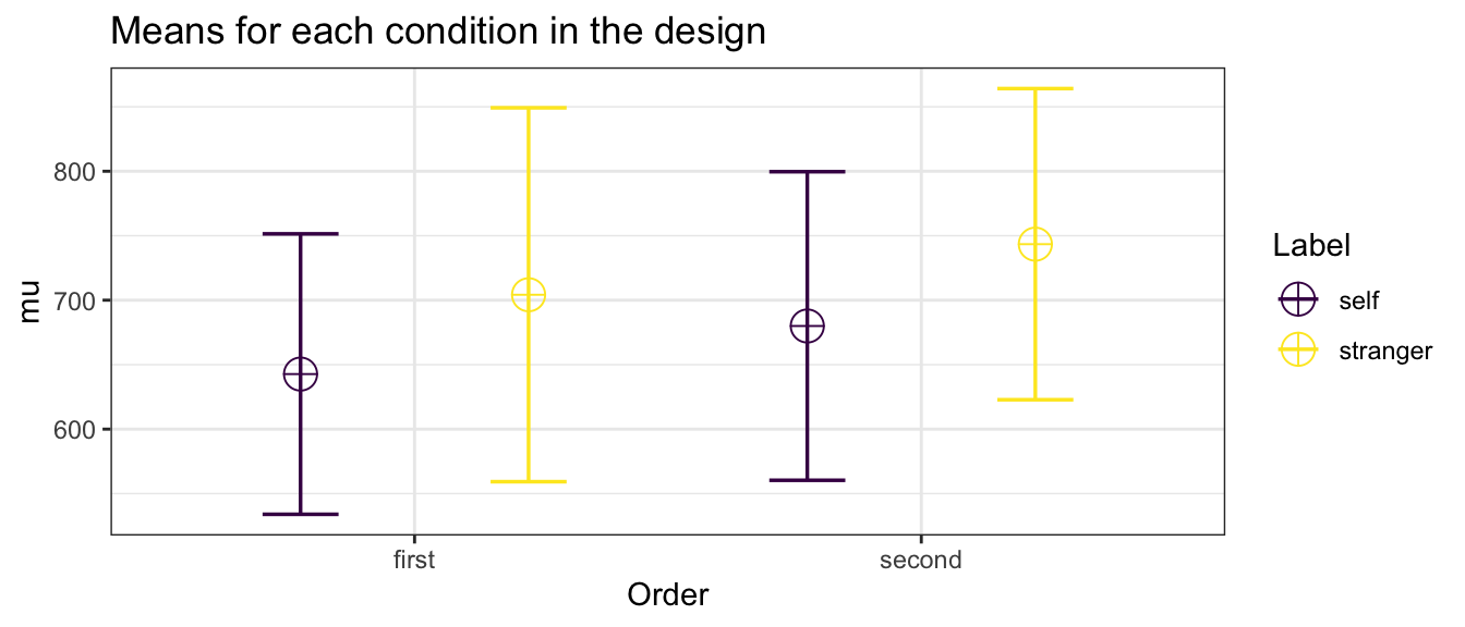
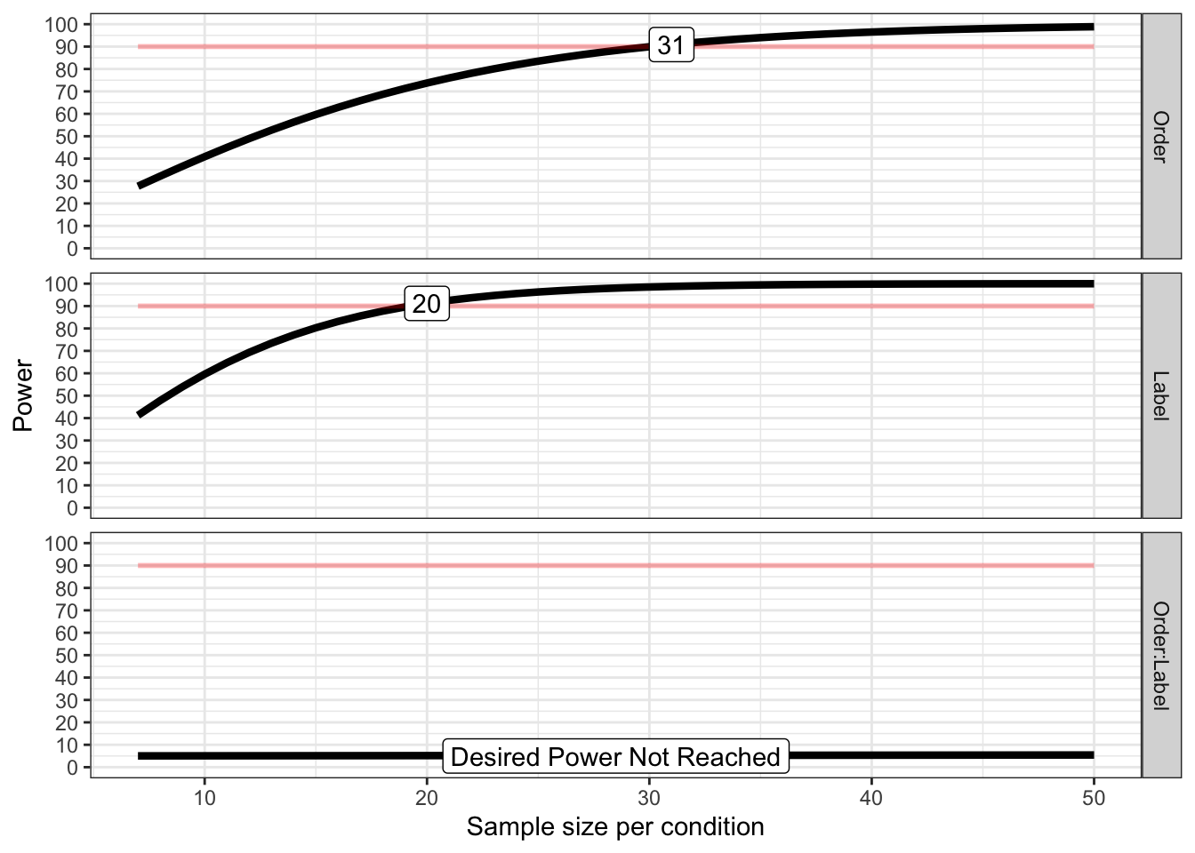
## Achieved Power and Sample Size for ANOVA-level effects
##      variable                     label  n achieved_power desired_power
## 1       Order    Desired Power Achieved 31          90.91            90
## 2       Label    Desired Power Achieved 20          91.18            90
## 3 Order:Label Desired Power Not Reached 50           5.44            90
The simulation results indicated that a minimum of 20 participants would be sufficient to detect the expected effect. To account for potential differences between our nonspatial WM task and Yin et al’s original task, we recruited 50% more participants, resulting in a total sample size of 30.
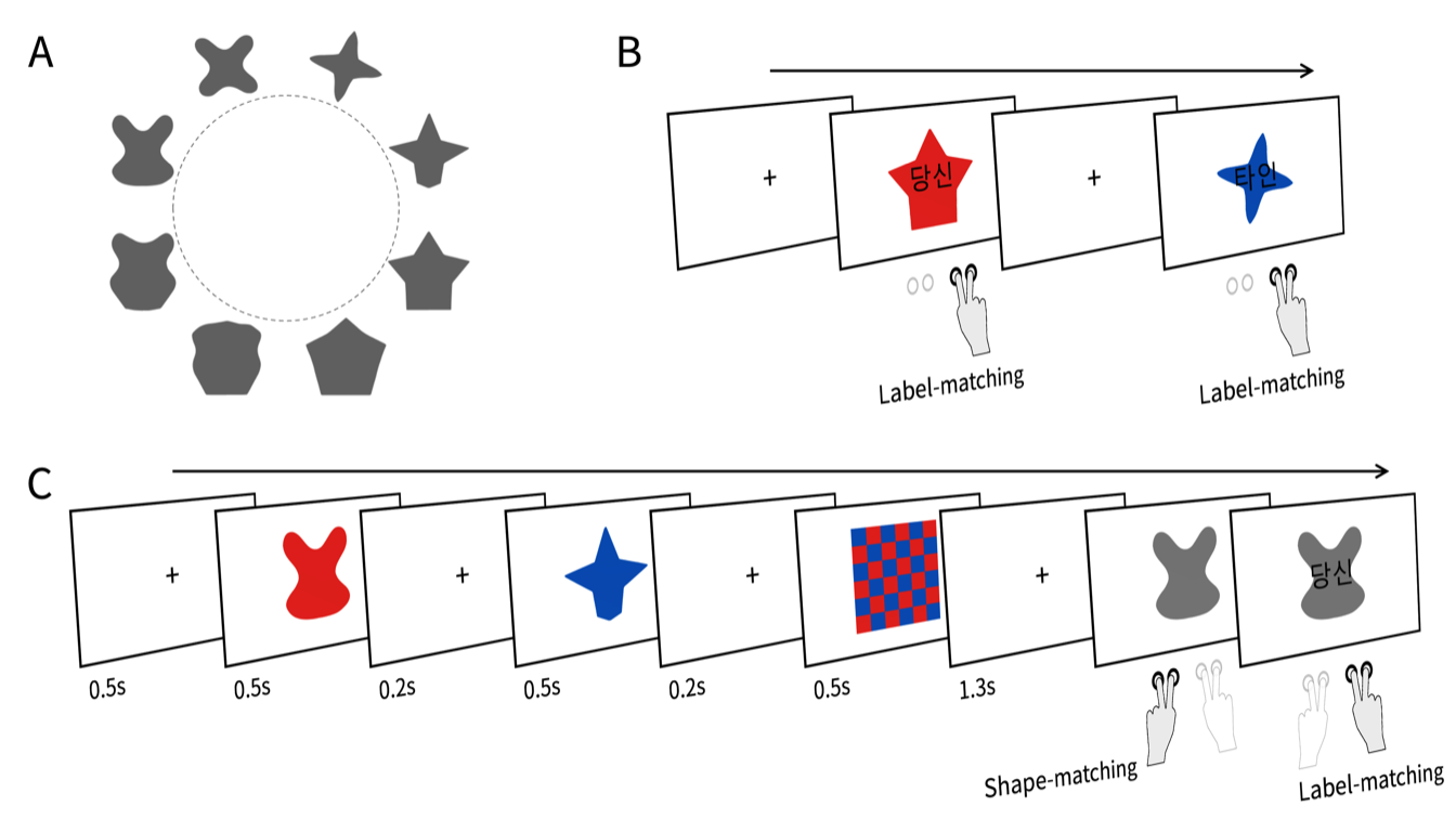
2 Stimuli & Tasks
Subjects completed an associative learning task followed by a working memory task.
The eight abstract shapes used in the tasks. These shapes were evenly sampled from the Validated Circular Shape (VCS) space (Li et al., 2020), designed to approximate the subjective similarity structure of the octagonal layout employed by Yin et al. (2019).
The figure shows two successive example trials in the associative learning task. Each trial presented a red or blue shape with a superimposed social label—“당신” (the Korean word for “you”) or “타인” (the Korean word for “stranger”). Subjects were asked to judge whether the shape color matched the color associated with the referent of the label (self or other) prior to the experiment. The shape’s form was irrelevant to the task and was included solely to familiarize subjects with the shapes used in the later working memory task. Subjects responded using their right hand by pressing a button corresponding to either “match” or “nonmatch.” We refer to this as the label-matching judgment.
Each trial of the working memory task presented a red shape, a blue shape, and a checkerboard pattern in sequence. In half of the trials, the red shape appeared first, and the blue shape appeared first in the other half. Subjects were required to briefly retain the samples’ colors and shapes in working memory. After a 1-second delay, a gray probe shape appeared on the screen, and subjects were asked to make a speeded and accurate judgment as to whether the probe matched either of the two previously presented samples. In 25% of the trials, the probe matched the first sample; in another 25%, it matched the second sample; and in the remaining 50%, it was a novel shape randomly drawn from the other six items in the shape set. Subjects responded using their left hand by pressing a button labeled “old” or “new.” We refer to this as the shape-matching response. On trials where the probe matched one of the two samples, a social label was superimposed on the probe immediately after the shape-matching response. Subjects were then asked to judge whether the color associated with the probed sample matched the color previously associated with the referent of the label (self or other). They responded using their right hand by pressing a button labeled “match” or “nonmatch.” We refer to this as another label-matching response.
3 Outlier Detection
We examined whether any of our subjects (N = 30) exhibited extreme performance that would warrant exclusion as outliers. Subjects made responses for label-color matching in the associative learning task, and for both shape-matching and label-color matching in the working memory task. For all three response types, we calculated each subject’s accuracy and mean response time (RT). Outlier subjects were identified using the boxplot method: a subject was classified as an outlier if their score on any of the six indices (three response types × accuracy and mean RT) exceeded Q3 + 3 × IQR or fell below Q1 – 3 × IQR.
Additionally, mean RTs were computed based only on correct responses, excluding values that deviated more than 2.5 standard deviations from the subject-specific mean.
In the raincloud plots below, each gray dot represents an individual subject’s performance across all trials. The red dashed line indicates the outlier cutoff at Q1 – 3 × IQR or Q3 + 3 × IQR, and the black dotted line marks Q1 – 1.5 × IQR or Q3 + 1.5 × IQR.
3.1 Learning Task: Label-Matching
# Data loading
s <- read.csv("data/datSPE8VCS1LRN.csv", header = T) %>%
  mutate(SN = factor(SN),
         Matching = factor(Matching,
                           labels = c("Match", "Nonmatch"),
                           levels = c("Match", "Nonmatch")),
         Label = factor(Label,
                        labels = c("Self", "Stranger"),
                        levels = c("Self", "Stranger")))
str(s)
## 'data.frame':    4320 obs. of  6 variables:
##  $ SN      : Factor w/ 30 levels "1","2","3","4",..: 1 1 1 1 1 1 1 1 1 1 ...
##  $ Matching: Factor w/ 2 levels "Match","Nonmatch": 1 2 1 1 2 2 1 1 1 2 ...
##  $ Label   : Factor w/ 2 levels "Self","Stranger": 1 1 1 1 1 2 2 1 2 2 ...
##  $ Response: chr  "Match" "Nonmatch" "Match" "Nonmatch" ...
##  $ Correct : int  1 1 1 0 1 1 0 1 0 1 ...
##  $ RT      : num  4161 1185 1289 871 2027 ...
headTail(s)
##        SN Matching    Label Response Correct     RT
## 1       1    Match     Self    Match       1 4161.4
## 2       1 Nonmatch     Self Nonmatch       1 1185.3
## 3       1    Match     Self    Match       1 1288.9
## 4       1    Match     Self Nonmatch       0  870.6
## ...  <NA>     <NA>     <NA>     <NA>     ...    ...
## 4317   30 Nonmatch Stranger Nonmatch       1 1323.8
## 4318   30 Nonmatch     Self Nonmatch       1  993.9
## 4319   30 Nonmatch Stranger Nonmatch       1 1732.4
## 4320   30 Nonmatch     Self    Match       0  828.4

# Accuracy summary
s.gc <- s %>%
  group_by(SN) %>%
  summarise(M = mean(Correct)) %>%
  ungroup()

s.gc %>% identify_outliers(M)
## # A tibble: 2 × 4
##   SN        M is.outlier is.extreme
##   <fct> <dbl> <lgl>      <lgl>
## 1 1     0.736 TRUE       TRUE
## 2 6     0.812 TRUE       FALSE

thresholds <- s.gc %>%
  summarise(Outlier = quantile(M, prob = .25) - 1.5 * IQR(M),
            Extreme = quantile(M, prob = .25) - 3 * IQR(M))
Fo1 <- s.gc %>%
  single_raincloud_plot(.$M, 0.5, 1, 0.1, "Label-Matching Accuracy") +
  geom_hline(yintercept=thresholds$Outlier, linetype="dotted") +
  geom_hline(yintercept=thresholds$Extreme, linetype='dashed', color='red', linewidth=0.5)

# RT (subject-wise trimming)
range(s$RT[s$Correct==1])
## [1]  327.1 4712.6

st <- s %>%
  filter(Correct == 1) %>%
  group_by(SN) %>%
  nest() %>%
  mutate(lbound = map(data, ~mean(.$RT)-tOff*sd(.$RT)),
         ubound = map(data, ~mean(.$RT)+tOff*sd(.$RT))) %>%
  unnest(c(lbound, ubound)) %>%
  unnest(data) %>%
  mutate(Outlier = (RT < lbound)|(RT > ubound)) %>%
  filter(Outlier == FALSE) %>%
  ungroup() %>%
  select(SN, Matching, Label,  RT)

range(st$RT)
## [1]  327.1 2955.4

# RT summary
s.gt <- st %>%
  group_by(SN) %>%
  summarise(M = mean(RT)) %>%
  ungroup()

s.gt %>% identify_outliers(M)
## # A tibble: 1 × 4
##   SN        M is.outlier is.extreme
##   <fct> <dbl> <lgl>      <lgl>
## 1 10    1175. TRUE       FALSE

# plot
thresholds <- s.gt %>%
  summarise(Outlier = quantile(M, prob = .75) + 1.5 * IQR(M),
            Extreme = quantile(M, prob = .75) + 3 * IQR(M))
Fo2 <- s.gt %>%
  single_raincloud_plot(.$M, 200, 1400, 200, "Label-Matching RTs (ms)") +
  geom_hline(yintercept=thresholds$Outlier, linetype="dotted") +
  geom_hline(yintercept=thresholds$Extreme, linetype='dashed', color='red', linewidth=0.5)

(Fo1 | Fo2) 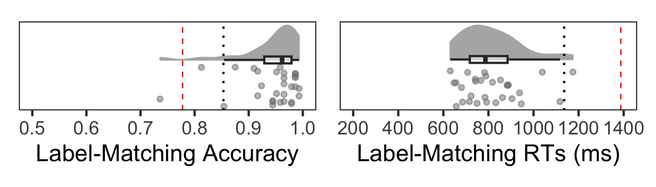
One subject (#1) showed outlier-level low accuracy. No subjects were excluded based on mean RT.
3.2 WM Task: Shape-Matching
Responses are correct if participants pressed the ‘Same’ key when the probe matched either sample shape, or the ‘Different’ key otherwise.
# Data loading
d <- read.csv("data/datSPE8VCS1TST.csv", header = T) %>%
  mutate(SN = factor(SN),
         Identity = factor(Identity,
                         labels = c("Self", "Stranger"),
                         levels = c("Self", "Stranger")),
         Order = factor(Order),
         Change = factor(Change),
         Matching = factor(Matching),
         Label = factor(Label,
                        labels = c("Self", "Stranger"),
                        levels = c("Self", "Stranger")))
str(d)
## 'data.frame':    8639 obs. of  10 variables:
##  $ SN      : Factor w/ 30 levels "1","2","3","4",..: 1 1 1 1 1 1 1 1 1 1 ...
##  $ Screen  : chr  "probe" "label" "probe" "label" ...
##  $ Identity: Factor w/ 2 levels "Self","Stranger": 1 1 2 2 2 2 1 1 2 2 ...
##  $ Order   : Factor w/ 3 levels "","First","Second": 3 3 2 2 3 3 2 2 3 3 ...
##  $ Change  : Factor w/ 2 levels "Different","Same": 2 2 2 2 2 2 2 2 2 2 ...
##  $ Matching: Factor w/ 3 levels "","Match","Nonmatch": 3 3 2 2 2 2 2 2 2 2 ...
##  $ Label   : Factor w/ 2 levels "Self","Stranger": 2 2 2 2 2 2 1 1 2 2 ...
##  $ Response: chr  "Same" "Nonmatch" "Same" "Match" ...
##  $ Correct : int  1 1 1 1 1 1 1 1 1 1 ...
##  $ RT      : num  865 789 1071 781 1054 ...
headTail(d)
##        SN Screen Identity  Order    Change Matching    Label  Response Correct
## 1       1  probe     Self Second      Same Nonmatch Stranger      Same       1
## 2       1  label     Self Second      Same Nonmatch Stranger  Nonmatch       1
## 3       1  probe Stranger  First      Same    Match Stranger      Same       1
## 4       1  label Stranger  First      Same    Match Stranger     Match       1
## ...  <NA>   <NA>     <NA>   <NA>      <NA>     <NA>     <NA>      <NA>     ...
## 8636   30  label Stranger  First      Same Nonmatch     Self  Nonmatch       1
## 8637   30  probe     Self  First      Same Nonmatch Stranger      Same       1
## 8638   30  label     Self  First      Same Nonmatch Stranger  Nonmatch       1
## 8639   30  probe     <NA>        Different              <NA> Different       1
##          RT
## 1     865.2
## 2     789.3
## 3    1071.5
## 4       781
## ...     ...
## 8636  927.2
## 8637  765.4
## 8638  730.8
## 8639  595.6

# Shape-matching judgments only
d.dms <- d %>%
  filter(Screen == "probe") %>%
  droplevels() %>%
  dplyr::select(!c(Screen, Identity, Order, Matching))

# Accuracy summary
dgc <- d.dms %>%
  group_by(SN) %>%
  summarise(M = mean(Correct)) %>%
  ungroup()

dgc %>% identify_outliers(M)
## [1] SN         M          is.outlier is.extreme
## <0 rows> (or 0-length row.names)

thresholds <- dgc %>%
  summarise(Outlier = quantile(M, prob = .25) - 1.5 * IQR(M),
            Extreme = quantile(M, prob = .25) - 3 * IQR(M))
Fo3 <- dgc %>%
  single_raincloud_plot(.$M, 0.5, 1, 0.1, "Shape-Matching Accuracy") +
  geom_hline(yintercept=thresholds$Outlier, linetype="dotted") +
  geom_hline(yintercept=thresholds$Extreme, linetype='dashed', color='red', linewidth=0.5)

# RT (subject-wise trimming)
range(d.dms$RT[d.dms$Correct==1])
## [1]   364.0 15223.3

dt <- d.dms %>%
  filter(Correct == 1) %>%
  group_by(SN) %>%
  nest() %>%
  mutate(lbound = map(data, ~mean(.$RT)-tOff*sd(.$RT)),
         ubound = map(data, ~mean(.$RT)+tOff*sd(.$RT))) %>%
  unnest(c(lbound, ubound)) %>%
  unnest(data) %>%
  mutate(Outlier = (RT < lbound)|(RT > ubound)) %>%
  filter(Outlier == FALSE) %>%
  ungroup %>%
  select(SN, Change, RT)

range(dt$RT)
## [1]  364.0 2520.6

# RT summary
dgt <- dt %>%
  group_by(SN) %>%
  summarise(M = mean(RT)) %>%
  ungroup()

dgt %>% identify_outliers(M)
## [1] SN         M          is.outlier is.extreme
## <0 rows> (or 0-length row.names)

thresholds <- dgt %>%
  summarise(Outlier = quantile(M, prob = .75) + 1.5 * IQR(M),
            Extreme = quantile(M, prob = .75) + 3 * IQR(M))
Fo4 <- dgt %>%
  single_raincloud_plot(.$M, 200, 1400, 200, "Shape-Matching RTs (ms)") +
  geom_hline(yintercept=thresholds$Outlier, linetype="dotted") +
  geom_hline(yintercept=thresholds$Extreme, linetype='dashed', color='red', linewidth=0.5)

(Fo3 | Fo4) 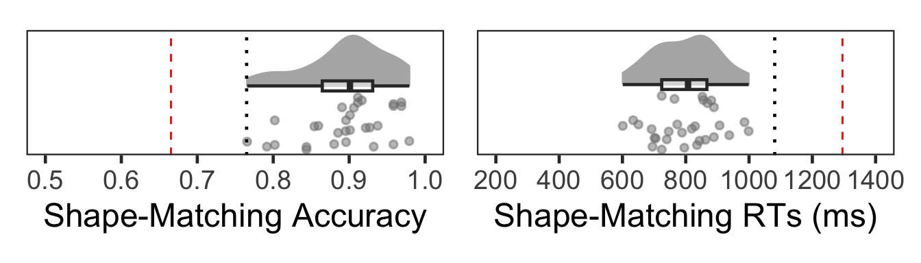
No subjects were identified as outliers based both on accuracy and on mean RTs.
3.3 WM Task: Label-Matching
# Label-color matching judgments only
d.spe <- d %>%
  filter(Screen == "label") %>% # label은 모두 Same
  droplevels() %>%
  select(!c(Screen, Identity, Order, Change))

# Accuracy summary
dgs <- d.spe %>%
  group_by(SN) %>%
  summarise(M = mean(Correct)) %>%
  ungroup()

dgs %>% identify_outliers(M)
## # A tibble: 2 × 4
##   SN        M is.outlier is.extreme
##   <fct> <dbl> <lgl>      <lgl>
## 1 6     0.656 TRUE       FALSE
## 2 10    0.688 TRUE       FALSE

thresholds <- dgs %>%
  summarise(Outlier = quantile(M, prob = .25) - 1.5 * IQR(M),
            Extreme = quantile(M, prob = .25) - 3 * IQR(M))
Fo5 <- dgs %>%
  single_raincloud_plot(.$M, 0.5, 1, 0.1, "WM Label-Matching Accuracy") +
  geom_hline(yintercept=thresholds$Outlier, linetype="dotted") +
  geom_hline(yintercept=thresholds$Extreme, linetype='dashed', color='red', linewidth=0.5)

# RT (subject-wise trimming)
range(d.spe$RT[d.spe$Correct==1])
## [1]  264.2 8908.2

d.spe.rt <- d.spe %>%
  filter(Correct == 1) %>%
  group_by(SN) %>%
  nest() %>%
  mutate(lbound = map(data, ~mean(.$RT)-tOff*sd(.$RT)),
         ubound = map(data, ~mean(.$RT)+tOff*sd(.$RT))) %>%
  unnest(c(lbound, ubound)) %>%
  unnest(data) %>%
  mutate(Outlier = (RT < lbound)|(RT > ubound)) %>%
  filter(Outlier == FALSE) %>%
  ungroup %>%
  select(SN, Matching, Label,  RT)

range(d.spe.rt$RT)
## [1]  264.2 3787.5

# RT summary
dptg <- d.spe.rt %>%
  group_by(SN) %>%
  summarise(M = mean(RT)) %>%
  ungroup()

dptg %>% identify_outliers(M)
## # A tibble: 3 × 4
##   SN        M is.outlier is.extreme
##   <fct> <dbl> <lgl>      <lgl>
## 1 10    1016. TRUE       FALSE
## 2 28     989. TRUE       FALSE
## 3 30    1320. TRUE       TRUE

thresholds <- dptg %>%
  summarise(OutlierL = quantile(M, prob = .25) - 1.5 * IQR(M),
            OutlierU = quantile(M, prob = .75) + 1.5 * IQR(M),
            Extreme = quantile(M, prob = .75) + 3 * IQR(M))
Fo6 <- dptg %>%
  single_raincloud_plot(.$M, 200, 1400, 200, "WM Label-Matching RTs (ms)") +
  geom_hline(yintercept=thresholds$OutlierL, linetype="dotted") +
  geom_hline(yintercept=thresholds$OutlierU, linetype="dotted") +
  geom_hline(yintercept=thresholds$Extreme, linetype='dashed', color='red', linewidth=0.5)

(Fo5 | Fo6)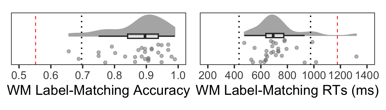
One subject (#30) was classified as an outlier due to slow mean RT.
excluded <- c(1, 30)

s <- rm_subject(s, excluded)
## 2 removed & 28 left
length(unique(s$SN))
## [1] 28

d <- rm_subject(d, excluded)
## 2 removed & 28 left
length(unique(d$SN))
## [1] 28
In summary, one subject with low label-matching accuracy in the associative learning task and another with markedly slow label-matching RT in the working memory task were classified as outliers and excluded from further analyses.
4 Associative Learning Task
4.1 Label-Matching Accuracy
In the following plots, self and stranger refer to labels. Note that in match trials, the shape’s color and label denote the same identity, whereas in nonmatch trials, the color and label denote different identities. Following prior research (Yin et al., 2019), self-bias was computed by comparing performance between the self and stranger conditions on match trials.
length(unique(s$SN))
## [1] 28
table(s$Label, s$SN)
##
##             2  3  4  5  6  7  8  9 10 11 12 13 14 15 16 17 18 19 20 21 22 23 24
##   Self     72 72 72 72 72 72 72 72 72 72 72 72 72 72 72 72 72 72 72 72 72 72 72
##   Stranger 72 72 72 72 72 72 72 72 72 72 72 72 72 72 72 72 72 72 72 72 72 72 72
##
##            25 26 27 28 29
##   Self     72 72 72 72 72
##   Stranger 72 72 72 72 72
table(s$Matching, s$SN)
##
##             2  3  4  5  6  7  8  9 10 11 12 13 14 15 16 17 18 19 20 21 22 23 24
##   Match    72 72 72 72 72 72 72 72 72 72 72 72 72 72 72 72 72 72 72 72 72 72 72
##   Nonmatch 72 72 72 72 72 72 72 72 72 72 72 72 72 72 72 72 72 72 72 72 72 72 72
##
##            25 26 27 28 29
##   Match    72 72 72 72 72
##   Nonmatch 72 72 72 72 72
table(s$Response, s$SN)
##
##             2  3  4  5  6  7  8  9 10 11 12 13 14 15 16 17 18 19 20 21 22 23 24
##   Match    76 78 71 73 77 74 72 69 73 73 66 72 72 74 72 71 71 69 73 76 68 71 69
##   Nonmatch 68 66 73 71 67 70 72 75 71 71 78 72 72 70 72 73 73 75 71 68 76 73 75
##
##            25 26 27 28 29
##   Match    73 74 70 69 73
##   Nonmatch 71 70 74 75 71
table(s$Correct, s$SN)
##
##       2   3   4   5   6   7   8   9  10  11  12  13  14  15  16  17  18  19  20
##   0   8  12   3   1  27  12   8   3   5   5   8   2   2   2  18   3   7  11   7
##   1 136 132 141 143 117 132 136 141 139 139 136 142 142 142 126 141 137 133 137
##
##      21  22  23  24  25  26  27  28  29
##   0   6   6   1   5  13   2   2   5   5
##   1 138 138 143 139 131 142 142 139 139

s.acc <- s %>%
  group_by(SN, Matching, Label) %>%
  summarise(Accuracy = mean(Correct)) %>%
  ungroup()

plotMatchLabel(s.acc, "Accuracy", 0.5, 1, .1, FALSE, -.1, .3, .1)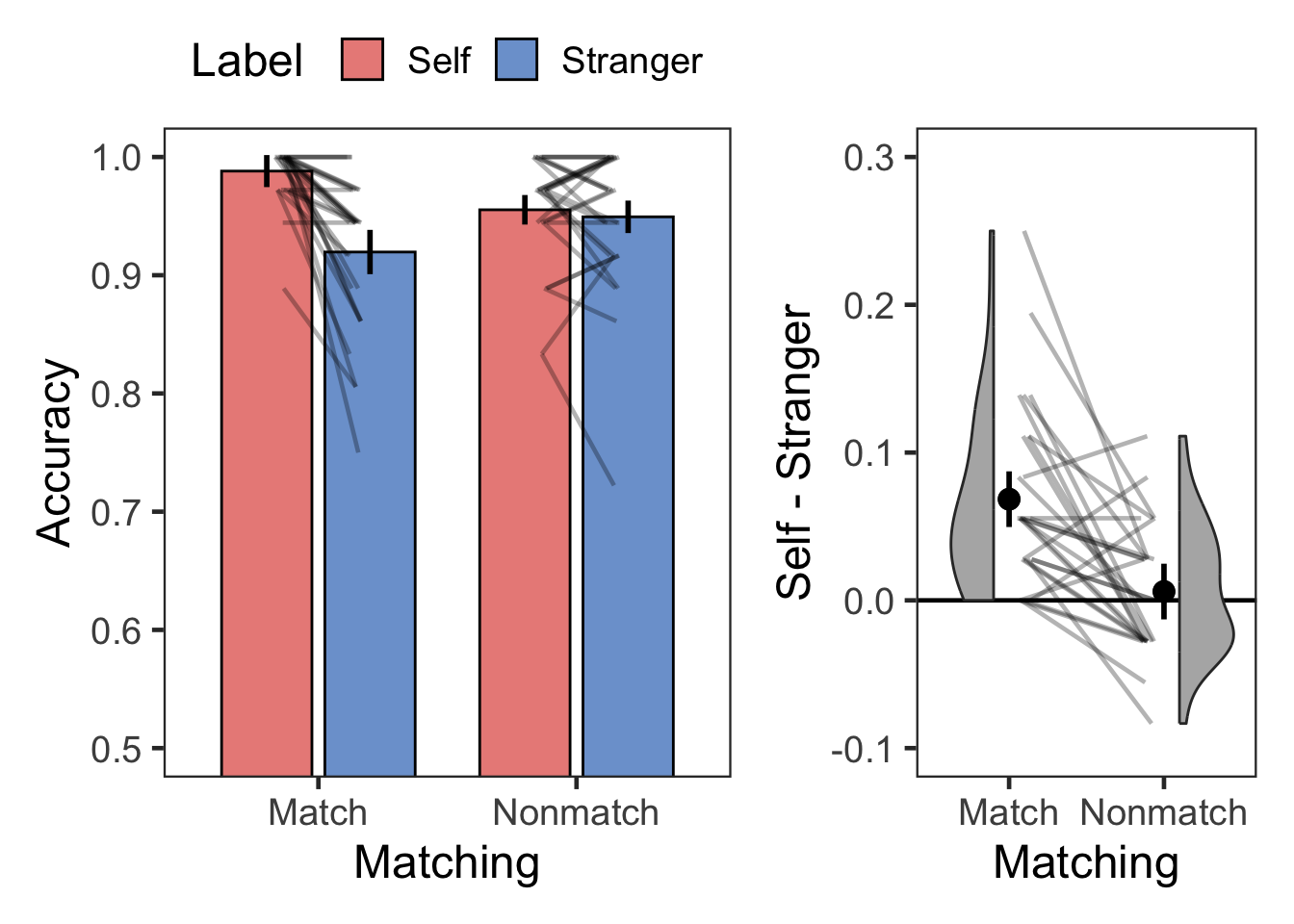
# Descriptive
s.acc %>% group_by(Matching, Label) %>%
  get_summary_stats(Accuracy, show = c("mean", "sd")) %>%
kable(digits = 2, format = "simple", caption = "Descriptive summary")| Matching | Label | variable | n | mean | sd |
|---|---|---|---|---|---|
| Match | Self | Accuracy | 28 | 0.99 | 0.02 |
| Match | Stranger | Accuracy | 28 | 0.92 | 0.06 |
| Nonmatch | Self | Accuracy | 28 | 0.96 | 0.05 |
| Nonmatch | Stranger | Accuracy | 28 | 0.95 | 0.06 |
# BF
( bf.sAcc <- anovaBF(Accuracy ~ Matching*Label + SN, data = as.data.frame(s.acc),
                     whichRandom = "SN", iterations = nIter, progress = FALSE) )
## Bayes factor analysis
## --------------
## [1] Matching + SN                          : 0.2020331 ±0.35%
## [2] Label + SN                             : 1835.635  ±0.7%
## [3] Matching + Label + SN                  : 376.8199  ±2.13%
## [4] Matching + Label + Matching:Label + SN : 173567.8  ±0.63%
##
## Against denominator:
##   Accuracy ~ SN
## ---
## Bayes factor type: BFlinearModel, JZS
# plot(bf.sAcc)

# ANOVA
cbind(
  anova_test(
    data = s.acc, dv = Accuracy, wid = SN,
    within = c(Matching, Label),
    effect.size = "pes") %>%
    get_anova_table(),
  tibble(BF10 = c( exp((bf.sAcc[3]/bf.sAcc[2])@bayesFactor$bf), # Matching
                   exp((bf.sAcc[3]/bf.sAcc[1])@bayesFactor$bf), # Label
                   exp((bf.sAcc[4]/bf.sAcc[3])@bayesFactor$bf) ), # Matching x Label
         BF01 = c( exp((bf.sAcc[2]/bf.sAcc[3])@bayesFactor$bf),
                   exp((bf.sAcc[1]/bf.sAcc[3])@bayesFactor$bf),
                   exp((bf.sAcc[3]/bf.sAcc[4])@bayesFactor$bf) ))) %>%
kable(digits = c(0,0,0,3,5,0,3,3,3), format = "simple", caption = "ANOVA")| Effect | DFn | DFd | F | p | p<.05 | pes | BF10 | BF01 |
|---|---|---|---|---|---|---|---|---|
| Matching | 1 | 27 | 0.042 | 0.83900 | 0.002 | 0.205 | 4.871 | |
| Label | 1 | 27 | 22.404 | 0.00006 | * | 0.453 | 1865.139 | 0.001 |
| Matching:Label | 1 | 27 | 23.160 | 0.00005 | * | 0.462 | 460.612 | 0.002 |
# Post-hoc
dgT <- 3
dgP <- 6
dgM <- 3
dgC <- 3
dgD <- 3
cbind(s.acc %>%
        group_by(Matching) %>%
        t_test(Accuracy ~ Label, ref.group = "Self",
               paired = TRUE, detailed = TRUE) %>%
        adjust_pvalue(method = "bonferroni") %>%
        add_significance("p.adj") %>%
        unite("Comparison", group1:group2, sep = " > ") %>%
        mutate("95% CI" = paste0("[", round(conf.low, digits = dgC), ", ",
                                 round(conf.high, digits = dgC), "]")) %>%
        rename('T' = statistic, M = estimate) %>%
        select(Matching, Comparison, 'T', df, p, p.adj, p.adj.signif,
               M, '95% CI'),
      s.acc %>%
        group_by(Matching) %>%
        cohens_d(Accuracy ~ Label, paired = TRUE, ref.group = "Self") %>%
        select("effsize", "magnitude") %>%
        rename("Cohen's d" = effsize)) %>%
  kable(digits = c(0,0,dgT,0,dgP,dgP,0,dgM,0,dgD,0),
format = "simple", caption = "T-Test, Bonferroni Corrected")| Matching | Comparison | T | df | p | p.adj | p.adj.signif | M | 95% CI | Cohen’s d | magnitude |
|---|---|---|---|---|---|---|---|---|---|---|
| Match | Self > Stranger | 5.832 | 27 | 0.000003 | 0.000007 | **** | 0.068 | [0.044, 0.093] | 1.102 | large |
| Nonmatch | Self > Stranger | 0.711 | 27 | 0.483000 | 0.966000 | ns | 0.006 | [-0.011, 0.023] | 0.134 | negligible |
4.2 Label-Matching RT
range(s$RT[s$Correct==1])
## [1]  327.1 4712.6

st <- s %>%
  filter(Correct == 1) %>%
  group_by(SN) %>%
  nest() %>%
  mutate(lbound = map(data, ~mean(.$RT)-tOff*sd(.$RT)),
         ubound = map(data, ~mean(.$RT)+tOff*sd(.$RT))) %>%
  unnest(c(lbound, ubound)) %>%
  unnest(data) %>%
  mutate(Outlier = (RT < lbound)|(RT > ubound)) %>%
  filter(Outlier == FALSE) %>%
  ungroup() %>%
  select(SN, Matching, Label,  RT)

range(st$RT)
## [1]  327.1 2955.4

# check numbers of trials per condition
tmp <- st %>%
  group_by(SN, Matching, Label) %>%
  summarise(n = n()) %>%
  ungroup()
range(tmp$n) # check min & max number of trials.
## [1] 25 36
tmp %>%
  unite("Cond", Matching:Label) %>%
  pivot_wider(id_cols = SN, names_from = Cond, values_from = n) %>%
  print(n = Inf) # relatively high accuracy. seems enough number of trials.
## # A tibble: 28 × 5
##    SN    Match_Self Match_Stranger Nonmatch_Self Nonmatch_Stranger
##    <fct>      <int>          <int>         <int>             <int>
##  1 2             36             32            32                31
##  2 3             34             34            29                33
##  3 4             36             33            33                35
##  4 5             36             35            34                34
##  5 6             32             27            30                25
##  6 7             36             30            30                33
##  7 8             35             32            34                32
##  8 9             36             31            35                36
##  9 10            36             33            33                32
## 10 11            36             33            35                32
## 11 12            35             30            35                33
## 12 13            36             33            35                33
## 13 14            36             34            34                36
## 14 15            35             36            32                35
## 15 16            36             27            31                31
## 16 17            35             34            35                32
## 17 18            33             33            34                35
## 18 19            35             29            34                32
## 19 20            35             34            34                32
## 20 21            36             35            33                29
## 21 22            36             31            33                35
## 22 23            36             34            35                34
## 23 24            36             30            35                33
## 24 25            35             31            31                32
## 25 26            36             35            35                33
## 26 27            36             34            35                33
## 27 28            35             33            34                35
## 28 29            35             34            34                33

( pTrim1 <- 100*(sum(s$Correct) - nrow(st))/sum(s$Correct) ) # proportion of the trimmed
## [1] 2.419984

# RT summary
s.rt <- st %>%
  group_by(SN, Matching, Label) %>%
  summarise(RT = mean(RT)) %>%
  ungroup()

plotMatchLabel(s.rt, "Response Time (ms)", 500, 1500, 200, TRUE, -200, 500, 100)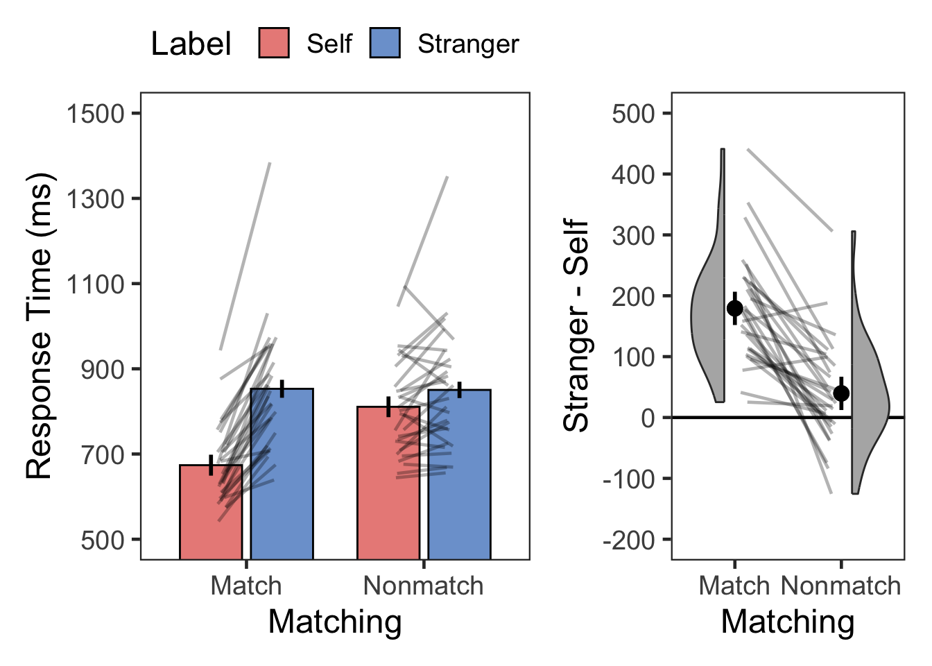
# Descriptive
s.rt %>% group_by(Matching, Label) %>%
  get_summary_stats(RT, show = c("mean", "sd")) %>%
kable(digits = 0, format = "simple", caption = "Descriptive summary")| Matching | Label | variable | n | mean | sd |
|---|---|---|---|---|---|
| Match | Self | RT | 28 | 674 | 93 |
| Match | Stranger | RT | 28 | 853 | 149 |
| Nonmatch | Self | RT | 28 | 811 | 116 |
| Nonmatch | Stranger | RT | 28 | 850 | 147 |
# BF
( bf.sRT <- anovaBF(RT ~ Matching*Label + SN, data = as.data.frame(s.rt),
                    whichRandom = "SN", iterations = nIter, progress = FALSE) )
## Bayes factor analysis
## --------------
## [1] Matching + SN                          : 77.65403          ±0.41%
## [2] Label + SN                             : 32084969          ±0.35%
## [3] Matching + Label + SN                  : 158872277832      ±0.61%
## [4] Matching + Label + Matching:Label + SN : 96469509162155792 ±1.08%
##
## Against denominator:
##   RT ~ SN
## ---
## Bayes factor type: BFlinearModel, JZS
# plot(bf.sRT)

# ANOVA
cbind(
  anova_test(
    data = s.rt, dv = RT, wid = SN,
    within = c(Matching, Label),
    effect.size = "pes") %>%
    get_anova_table() ,
  tibble(BF10 = c( exp((bf.sRT[3]/bf.sRT[2])@bayesFactor$bf),
                   exp((bf.sRT[3]/bf.sRT[1])@bayesFactor$bf),
                   exp((bf.sRT[4]/bf.sRT[3])@bayesFactor$bf) ),
         BF01 = c( exp((bf.sRT[2]/bf.sRT[3])@bayesFactor$bf),
                   exp((bf.sRT[1]/bf.sRT[3])@bayesFactor$bf),
                   exp((bf.sRT[3]/bf.sRT[4])@bayesFactor$bf) ))) %>%
kable(digits = c(0,0,0,3,9,0,3,3,3), format = "simple", caption = "ANOVA")| Effect | DFn | DFd | F | p | p<.05 | pes | BF10 | BF01 |
|---|---|---|---|---|---|---|---|---|
| Matching | 1 | 27 | 67.373 | 0.000000008 | * | 0.714 | 4951.611 | 0 |
| Label | 1 | 27 | 59.443 | 0.000000027 | * | 0.688 | 2045898660.836 | 0 |
| Matching:Label | 1 | 27 | 54.859 | 0.000000057 | * | 0.670 | 607214.238 | 0 |
# Post-hoc
dgT <- 3
dgP <- 11
dgM <- 0
dgC <- 0
dgD <- 3
cbind(s.rt %>%
        group_by(Matching) %>%
        t_test(RT ~ Label, ref.group = "Stranger",
               paired = TRUE, detailed = TRUE) %>%
        adjust_pvalue(method = "bonferroni") %>%
        add_significance("p.adj") %>%
        unite("Comparison", group1:group2, sep = " > ") %>%
        mutate("95% CI" = paste0("[", round(conf.low, digits = dgC), ", ",
                                 round(conf.high, digits = dgC), "]")) %>%
        rename('T' = statistic, M = estimate) %>%
        select(Matching, Comparison, 'T', df, p, p.adj, p.adj.signif,
               M, '95% CI'),
      s.rt %>%
        group_by(Matching) %>%
        cohens_d(RT ~ Label, paired = TRUE, ref.group = "Stranger") %>%
        select("effsize", "magnitude") %>%
        rename("Cohen's d" = effsize)) %>%
  kable(digits = c(0,0,dgT,0,dgP,dgP,0,dgM,0,dgD,0),
format = "simple", caption = "T-Test, Bonferroni Corrected")| Matching | Comparison | T | df | p | p.adj | p.adj.signif | M | 95% CI | Cohen’s d | magnitude |
|---|---|---|---|---|---|---|---|---|---|---|
| Match | Stranger > Self | 10.238 | 27 | 0.00000000009 | 0.00000000017 | **** | 179 | [143, 215] | 1.935 | large |
| Nonmatch | Stranger > Self | 2.394 | 27 | 0.02390000000 | 0.04780000000 | * | 40 | [6, 74] | 0.452 | small |
2.42% of RTs were removed as extreme values.
5 Working Memory Task
5.1 DMS Accuracy & RT
The delayed match-to-sample judgment was analyzed by dividing the trials into same trials, where the probe matched one of the two samples, and Different trials, where the probe matched neither sample.
dc <- d %>% filter(Screen == "probe") %>%
  droplevels() %>%
  select(!c(Screen, Matching, Label, Identity, Response, Order))
table(dc$Change, dc$Correct)
##
##                0    1
##   Different  286 2401
##   Same       279 2409

rbind(
  dc %>%
    group_by(SN) %>%
    summarise(M = mean(Correct)) %>%
    ungroup() %>%
    summarise(Mean = mean(M), SD = sd(M)) %>%
    mutate(Change = factor("Overall")) %>%
    select(Change, Mean, SD),
  dc %>%
    group_by(SN, Change) %>%
    summarise(M = mean(Correct)) %>%
    ungroup() %>%
    group_by(Change) %>%
    summarise(Mean = mean(M), SD = sd(M))) %>%
  pivot_longer(cols = -Change, names_to = "Statistic", values_to = "Value") %>%
  pivot_wider(names_from = Change, values_from = Value) %>%
  select(Statistic, Overall, Same, Different) %>%
  kable(digits = c(0,3,3,3),
format = "simple", caption = "DMS Judgment Summary")| Statistic | Overall | Same | Different |
|---|---|---|---|
| Mean | 0.895 | 0.896 | 0.894 |
| SD | 0.057 | 0.073 | 0.054 |
5.2 Shape-Matching Accuracy
The key dependent measure was RT on correct shape-probe-match trials, referring to trials where the probe matched one of the two sample shapes in working memory (Yin et al.).
Shape-matching responses were classified according to two factors: identity and order. Identity refers to the social label associated with the color of the sample that matched the probe shape. Note that no labels were presented on the screen when these responses were collected. Order indicates whether the sample shape that matched the probe appeared first or second.
In this task, self-bias was defined as the difference in performance between the self and stranger conditions, averaged across the two order conditions.
d.same <- d %>%
  filter(Change == "Same", Screen == "probe") %>%
  droplevels() %>%
  select(!c(Screen, Change, Matching, Label))
str(d.same)
## 'data.frame':    2688 obs. of  6 variables:
##  $ SN      : Factor w/ 28 levels "2","3","4","5",..: 1 1 1 1 1 1 1 1 1 1 ...
##  $ Identity: Factor w/ 2 levels "Self","Stranger": 2 2 2 2 2 1 2 2 1 1 ...
##  $ Order   : Factor w/ 2 levels "First","Second": 2 1 2 1 1 2 1 2 2 2 ...
##  $ Response: chr  "Different" "Same" "Same" "Same" ...
##  $ Correct : int  0 1 1 1 1 1 1 1 1 1 ...
##  $ RT      : num  808 893 857 933 1094 ...
table(d.same$SN)
##
##  2  3  4  5  6  7  8  9 10 11 12 13 14 15 16 17 18 19 20 21 22 23 24 25 26 27
## 96 96 96 96 96 96 96 96 96 96 96 96 96 96 96 96 96 96 96 96 96 96 96 96 96 96
## 28 29
## 96 96
table(d.same$Identity, d.same$SN)
##
##             2  3  4  5  6  7  8  9 10 11 12 13 14 15 16 17 18 19 20 21 22 23 24
##   Self     48 48 48 48 48 48 48 48 48 48 48 48 48 48 48 48 48 48 48 48 48 48 48
##   Stranger 48 48 48 48 48 48 48 48 48 48 48 48 48 48 48 48 48 48 48 48 48 48 48
##
##            25 26 27 28 29
##   Self     48 48 48 48 48
##   Stranger 48 48 48 48 48
table(d.same$Order, d.same$SN)
##
##           2  3  4  5  6  7  8  9 10 11 12 13 14 15 16 17 18 19 20 21 22 23 24
##   First  48 48 48 48 48 48 48 48 48 48 48 48 48 48 48 48 48 48 48 48 48 48 48
##   Second 48 48 48 48 48 48 48 48 48 48 48 48 48 48 48 48 48 48 48 48 48 48 48
##
##          25 26 27 28 29
##   First  48 48 48 48 48
##   Second 48 48 48 48 48
table(d.same$Response, d.same$SN)
##
##              2  3  4  5  6  7  8  9 10 11 12 13 14 15 16 17 18 19 20 21 22 23
##   Different  1 16  1  3 17 14 25  8 22  7 10  1  6  6  4 20 12 13  3  9 11 16
##   Same      95 80 95 93 79 82 71 88 74 89 86 95 90 90 92 76 84 83 93 87 85 80
##
##             24 25 26 27 28 29
##   Different 10 23  4  5  9  3
##   Same      86 73 92 91 87 93
table(d.same$Correct, d.same$SN)
##
##      2  3  4  5  6  7  8  9 10 11 12 13 14 15 16 17 18 19 20 21 22 23 24 25 26
##   0  1 16  1  3 17 14 25  8 22  7 10  1  6  6  4 20 12 13  3  9 11 16 10 23  4
##   1 95 80 95 93 79 82 71 88 74 89 86 95 90 90 92 76 84 83 93 87 85 80 86 73 92
##
##     27 28 29
##   0  5  9  3
##   1 91 87 93

# Shape-probe-match accuracy
dsa <- d.same %>%
  group_by(SN, Order, Identity) %>%
  summarise(Accuracy = mean(Correct)) %>%
  ungroup()

plotOrderIdentity(dsa, "Accuracy", 0.5, 1, .1, FALSE, -.2, .3, .1, .1)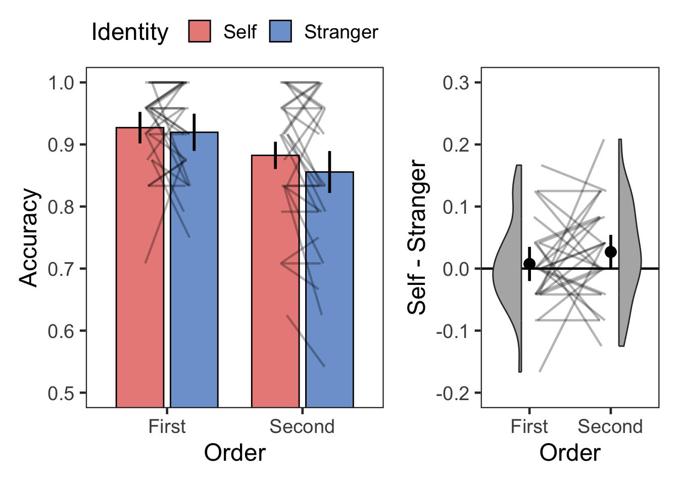
# Descriptive
dsa %>% group_by(Order, Identity) %>%
  get_summary_stats(Accuracy, show = c("mean", "sd")) %>%
kable(digits = 2, format = "simple", caption = "Descriptive summary")| Order | Identity | variable | n | mean | sd |
|---|---|---|---|---|---|
| First | Self | Accuracy | 28 | 0.93 | 0.07 |
| First | Stranger | Accuracy | 28 | 0.92 | 0.07 |
| Second | Self | Accuracy | 28 | 0.88 | 0.10 |
| Second | Stranger | Accuracy | 28 | 0.86 | 0.13 |
# BF
( bf.dAcc <- anovaBF(Accuracy ~ Order*Identity + SN, data = as.data.frame(dsa),
                     whichRandom = "SN", iterations = nIter, progress = FALSE) )
## Bayes factor analysis
## --------------
## [1] Order + SN                             : 149.9328  ±0.16%
## [2] Identity + SN                          : 0.3634671 ±0.31%
## [3] Order + Identity + SN                  : 60.54297  ±0.4%
## [4] Order + Identity + Order:Identity + SN : 19.97899  ±0.82%
##
## Against denominator:
##   Accuracy ~ SN
## ---
## Bayes factor type: BFlinearModel, JZS

# ANOVA
cbind(
  anova_test(
    data = dsa, dv = Accuracy, wid = SN,
    within = c(Order, Identity),
    effect.size = "pes") %>%
    get_anova_table() ,
  tibble(BF10 = c( exp((bf.dAcc[3]/bf.dAcc[2])@bayesFactor$bf),
                   exp((bf.dAcc[3]/bf.dAcc[1])@bayesFactor$bf),
                   exp((bf.dAcc[4]/bf.dAcc[3])@bayesFactor$bf) ),
         BF01 = c( exp((bf.dAcc[2]/bf.dAcc[3])@bayesFactor$bf),
                   exp((bf.dAcc[1]/bf.dAcc[3])@bayesFactor$bf),
                   exp((bf.dAcc[3]/bf.dAcc[4])@bayesFactor$bf) ))) %>%
kable(digits = c(0,0,0,3,3,0,3,3,3), format = "simple", caption = "ANOVA")| Effect | DFn | DFd | F | p | p<.05 | pes | BF10 | BF01 |
|---|---|---|---|---|---|---|---|---|
| Order | 1 | 27 | 8.174 | 0.008 | * | 0.232 | 166.571 | 0.006 |
| Identity | 1 | 27 | 2.601 | 0.118 | 0.088 | 0.404 | 2.476 | |
| Order:Identity | 1 | 27 | 1.038 | 0.317 | 0.037 | 0.330 | 3.030 |
# Post-hoc
dgT <- 3
dgP <- 3
dgM <- 3
dgC <- 3
dgD <- 3
cbind(dsa %>%
        group_by(Order) %>%
        t_test(Accuracy ~ Identity, ref.group = "Self",
               paired = TRUE, detailed = TRUE) %>%
        adjust_pvalue(method = "bonferroni") %>%
        add_significance("p.adj") %>%
        unite("Comparison", group1:group2, sep = " > ") %>%
        mutate("95% CI" = paste0("[", round(conf.low, digits = dgC), ", ",
                                 round(conf.high, digits = dgC), "]")) %>%
        rename('T' = statistic, M = estimate) %>%
        select(Order, Comparison, 'T', df, p, p.adj, p.adj.signif,
               M, '95% CI'),
      dsa %>%
        group_by(Order) %>%
        cohens_d(Accuracy ~ Identity, paired = TRUE, ref.group = "Self") %>%
        select("effsize", "magnitude") %>%
        rename("Cohen's d" = effsize)) %>%
  kable(digits = c(0,0,dgT,0,dgP,dgP,0,dgM,0,dgD,0),
format = "simple", caption = "T-Test, Bonferroni Corrected")| Order | Comparison | T | df | p | p.adj | p.adj.signif | M | 95% CI | Cohen’s d | magnitude |
|---|---|---|---|---|---|---|---|---|---|---|
| First | Self > Stranger | 0.542 | 27 | 0.592 | 1.00 | ns | 0.007 | [-0.021, 0.036] | 0.102 | negligible |
| Second | Self > Stranger | 1.819 | 27 | 0.080 | 0.16 | ns | 0.027 | [-0.003, 0.057] | 0.344 | small |
5.3 Shape-Matching RT
range(d.same$RT[d.same$Correct==1])
## [1]   364.0 15223.3

d.same.rt <- d.same %>%
  filter(Correct == 1) %>%
  group_by(SN) %>%
  nest() %>%
  mutate(lbound = map(data, ~mean(.$RT)-tOff*sd(.$RT)),
         ubound = map(data, ~mean(.$RT)+tOff*sd(.$RT))) %>%
  unnest(c(lbound, ubound)) %>%
  unnest(data) %>%
  mutate(Outlier = (RT < lbound)|(RT > ubound)) %>%
  filter(Outlier == FALSE) %>%
  ungroup %>%
  select(SN, Identity, Order, RT)

range(d.same.rt$RT)
## [1]  364.0 2018.5

# check numbers of trials per condition
tmp <- d.same.rt %>%
  group_by(SN, Order, Identity) %>%
  summarise(n = n()) %>%
  ungroup()
range(tmp$n) # check min & max number of trials
## [1] 11 24
tmp %>%
  unite("Cond", Order:Identity) %>%
  pivot_wider(id_cols = SN, names_from = Cond, values_from = n) %>%
  print(n = Inf) # SN 25 had only 11 trials.
## # A tibble: 28 × 5
##    SN    First_Self First_Stranger Second_Self Second_Stranger
##    <fct>      <int>          <int>       <int>           <int>
##  1 2             24             22          24              23
##  2 3             20             21          20              17
##  3 4             24             24          23              22
##  4 5             22             21          24              22
##  5 6             21             17          20              20
##  6 7             23             23          17              18
##  7 8             16             21          17              15
##  8 9             23             24          21              19
##  9 10            17             20          17              16
## 10 11            22             24          21              20
## 11 12            21             24          20              19
## 12 13            24             22          23              24
## 13 14            21             22          22              24
## 14 15            22             22          21              24
## 15 16            23             21          24              22
## 16 17            20             20          19              15
## 17 18            21             20          20              22
## 18 19            22             21          19              19
## 19 20            23             24          23              21
## 20 21            23             22          21              19
## 21 22            24             19          22              18
## 22 23            21             20          20              17
## 23 24            22             16          23              21
## 24 25            23             21          14              11
## 25 26            22             21          23              24
## 26 27            23             24          22              19
## 27 28            20             21          20              23
## 28 29            21             23          23              24

( pTrim3 <- 100*(sum(d.same$Correct) - nrow(d.same.rt))/sum(d.same$Correct)) # proportion of trimmed RTs
## [1] 2.49066

dst <- d.same.rt %>%
  group_by(SN, Order, Identity) %>%
  summarise(RT = mean(RT)) %>%
  ungroup()

plotOrderIdentity(dst, "Response Time (ms)", 500, 1300, 200, TRUE, -150, 200, 50, 1)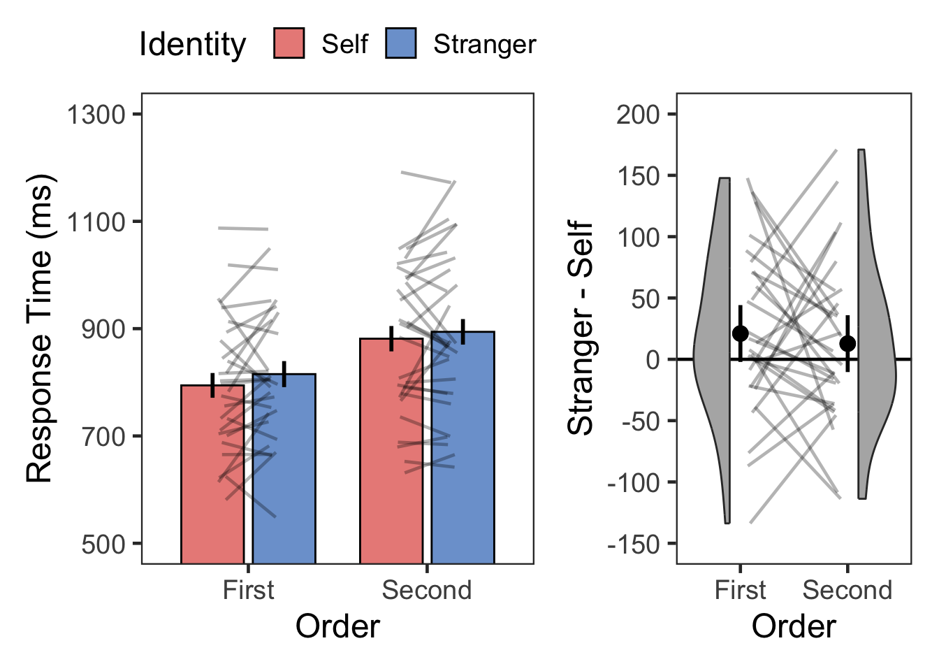
# Descriptive
dst %>% group_by(Order, Identity) %>%
  get_summary_stats(RT, show = c("mean", "sd")) %>%
kable(digits = 0, format = "simple", caption = "Descriptive summary")| Order | Identity | variable | n | mean | sd |
|---|---|---|---|---|---|
| First | Self | RT | 28 | 794 | 128 |
| First | Stranger | RT | 28 | 815 | 128 |
| Second | Self | RT | 28 | 881 | 142 |
| Second | Stranger | RT | 28 | 894 | 155 |
# BF
( bf.dRT <- anovaBF(RT ~ Order*Identity + SN, data = as.data.frame(dst),
                    whichRandom = "SN", iterations = nIter, progress = FALSE) )
## Bayes factor analysis
## --------------
## [1] Order + SN                             : 23841276  ±0.3%
## [2] Identity + SN                          : 0.3630282 ±0.4%
## [3] Order + Identity + SN                  : 12536807  ±2.08%
## [4] Order + Identity + Order:Identity + SN : 3570318   ±2.54%
##
## Against denominator:
##   RT ~ SN
## ---
## Bayes factor type: BFlinearModel, JZS
# plot(bf.dAcc)

# ANOVA
cbind(
  anova_test(
    data = dst, dv = RT, wid = SN,
    within = c(Order, Identity),
    effect.size = "pes") %>%
    get_anova_table() ,
  tibble(BF10 = c( exp((bf.dRT[3]/bf.dRT[2])@bayesFactor$bf),
                   exp((bf.dRT[3]/bf.dRT[1])@bayesFactor$bf),
                   exp((bf.dRT[4]/bf.dRT[3])@bayesFactor$bf) ),
         BF01 = c( exp((bf.dRT[2]/bf.dRT[3])@bayesFactor$bf),
                   exp((bf.dRT[1]/bf.dRT[3])@bayesFactor$bf),
                   exp((bf.dRT[3]/bf.dRT[4])@bayesFactor$bf) ))) %>%
kable(digits = c(0,0,0,3,9,0,3,3,3), format = "simple", caption = "ANOVA")| Effect | DFn | DFd | F | p | p<.05 | pes | BF10 | BF01 |
|---|---|---|---|---|---|---|---|---|
| Order | 1 | 27 | 29.375 | 0.00000988 | * | 0.521 | 34533977.251 | 0.000 |
| Identity | 1 | 27 | 2.802 | 0.10600000 | 0.094 | 0.526 | 1.902 | |
| Order:Identity | 1 | 27 | 0.266 | 0.61000000 | 0.010 | 0.285 | 3.511 |
# Post-hoc
dgT <- 3
dgP <- 11
dgM <- 0
dgC <- 0
dgD <- 3
cbind(dst %>%
        group_by(Order) %>%
        t_test(RT ~ Identity, ref.group = "Stranger",
               paired = TRUE, detailed = TRUE) %>%
        adjust_pvalue(method = "bonferroni") %>%
        add_significance("p.adj") %>%
        unite("Comparison", group1:group2, sep = " > ") %>%
        mutate("95% CI" = paste0("[", round(conf.low, digits = dgC), ", ",
                                 round(conf.high, digits = dgC), "]")) %>%
        rename('T' = statistic, M = estimate) %>%
        select(Order, Comparison, 'T', df, p, p.adj, p.adj.signif,
               M, '95% CI'),
      dst %>%
        group_by(Order) %>%
        cohens_d(RT ~ Identity, paired = TRUE, ref.group = "Stranger") %>%
        select("effsize", "magnitude") %>%
        rename("Cohen's d" = effsize)) %>%
  kable(digits = c(0,0,dgT,0,dgP,dgP,0,dgM,0,dgD,0),
format = "simple", caption = "T-Test, Bonferroni Corrected")| Order | Comparison | T | df | p | p.adj | p.adj.signif | M | 95% CI | Cohen’s d | magnitude |
|---|---|---|---|---|---|---|---|---|---|---|
| First | Stranger > Self | 1.637 | 27 | 0.113 | 0.226 | ns | 21 | [-5, 47] | 0.309 | small |
| Second | Stranger > Self | 0.991 | 27 | 0.331 | 0.662 | ns | 13 | [-14, 39] | 0.187 | negligible |
2.49% of RTs were removed as extreme values.
5.4 Label-Matching Accuracy
The same analytic procedure as in the associative learning task was applied.
d.spe <- d %>%
  filter(Screen == "label") %>% # label은 모두 Same
  droplevels() %>%
  select(!c(Screen, Identity, Order, Change))
str(d.spe)
## 'data.frame':    2688 obs. of  6 variables:
##  $ SN      : Factor w/ 28 levels "2","3","4","5",..: 1 1 1 1 1 1 1 1 1 1 ...
##  $ Matching: Factor w/ 2 levels "Match","Nonmatch": 1 1 2 2 1 2 1 2 2 1 ...
##  $ Label   : Factor w/ 2 levels "Self","Stranger": 2 2 1 1 2 2 2 1 2 1 ...
##  $ Response: chr  "Match" "Match" "Nonmatch" "Nonmatch" ...
##  $ Correct : int  1 1 1 1 1 1 1 1 0 1 ...
##  $ RT      : num  1790 569 689 810 1025 ...
table(d.spe$Matching, d.spe$SN)
##
##             2  3  4  5  6  7  8  9 10 11 12 13 14 15 16 17 18 19 20 21 22 23 24
##   Match    48 48 48 48 48 48 48 48 48 48 48 48 48 48 48 48 48 48 48 48 48 48 48
##   Nonmatch 48 48 48 48 48 48 48 48 48 48 48 48 48 48 48 48 48 48 48 48 48 48 48
##
##            25 26 27 28 29
##   Match    48 48 48 48 48
##   Nonmatch 48 48 48 48 48
table(d.spe$Label, d.spe$SN)
##
##             2  3  4  5  6  7  8  9 10 11 12 13 14 15 16 17 18 19 20 21 22 23 24
##   Self     48 48 48 48 48 48 48 48 48 48 48 48 48 48 48 48 48 48 48 48 48 48 48
##   Stranger 48 48 48 48 48 48 48 48 48 48 48 48 48 48 48 48 48 48 48 48 48 48 48
##
##            25 26 27 28 29
##   Self     48 48 48 48 48
##   Stranger 48 48 48 48 48
table(d.spe$Response, d.spe$SN)
##
##             2  3  4  5  6  7  8  9 10 11 12 13 14 15 16 17 18 19 20 21 22 23 24
##   Match    48 53 49 49 61 50 58 40 52 43 46 43 48 47 42 51 51 50 42 47 51 47 48
##   Nonmatch 48 43 47 47 35 46 38 56 44 53 50 53 48 49 54 45 45 46 54 49 45 49 48
##
##            25 26 27 28 29
##   Match    58 48 46 45 51
##   Nonmatch 38 48 50 51 45
table(d.spe$Correct, d.spe$SN)
##
##      2  3  4  5  6  7  8  9 10 11 12 13 14 15 16 17 18 19 20 21 22 23 24 25 26
##   0  2  9  3  1 33 10 24  8 30  5 20  5  6 13 12 11  9 22 16  3  5 19  6 24  8
##   1 94 87 93 95 63 86 72 88 66 91 76 91 90 83 84 85 87 74 80 93 91 77 90 72 88
##
##     27 28 29
##   0 10 13  9
##   1 86 83 87

# Accuracy
dgs <- d.spe %>%
  group_by(SN, Matching, Label) %>%
  summarise(Accuracy = mean(Correct)) %>%
  ungroup()

plotMatchLabel(dgs, "Accuracy", 0.5, 1, .1, FALSE, -.2, .4, .1)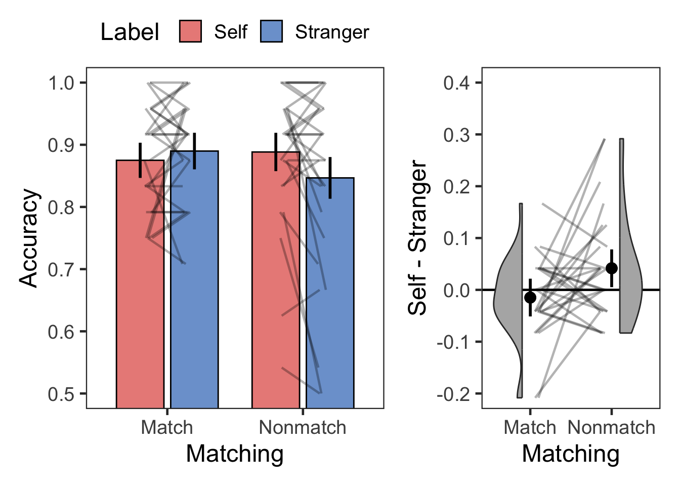
# Descriptive
dgs %>% group_by(Matching, Label) %>%
  get_summary_stats(Accuracy, show = c("mean", "sd")) %>%
kable(digits = 2, format = "simple", caption = "Descriptive summary")| Matching | Label | variable | n | mean | sd |
|---|---|---|---|---|---|
| Match | Self | Accuracy | 28 | 0.88 | 0.09 |
| Match | Stranger | Accuracy | 28 | 0.89 | 0.09 |
| Nonmatch | Self | Accuracy | 28 | 0.89 | 0.11 |
| Nonmatch | Stranger | Accuracy | 28 | 0.85 | 0.15 |
# BF
( bf.dSpeAcc <- anovaBF(Accuracy ~ Matching*Label + SN, data = as.data.frame(dgs),
                        whichRandom = "SN", iterations = nIter, progress = FALSE) )
## Bayes factor analysis
## --------------
## [1] Matching + SN                          : 0.3058686  ±0.21%
## [2] Label + SN                             : 0.3048416  ±3.72%
## [3] Matching + Label + SN                  : 0.08694748 ±0.54%
## [4] Matching + Label + Matching:Label + SN : 0.1124716  ±2.9%
##
## Against denominator:
##   Accuracy ~ SN
## ---
## Bayes factor type: BFlinearModel, JZS
# plot(bf.dSpeAcc)

# ANOVA
cbind(
  anova_test(
    data = dgs, dv = Accuracy, wid = SN,
    within = c(Matching, Label),
    effect.size = "pes") %>%
    get_anova_table() ,
  tibble(BF10 = c( exp((bf.dSpeAcc[3]/bf.dSpeAcc[2])@bayesFactor$bf),
                   exp((bf.dSpeAcc[3]/bf.dSpeAcc[1])@bayesFactor$bf),
                   exp((bf.dSpeAcc[4]/bf.dSpeAcc[3])@bayesFactor$bf) ),
         BF01 = c( exp((bf.dSpeAcc[2]/bf.dSpeAcc[3])@bayesFactor$bf),
                   exp((bf.dSpeAcc[1]/bf.dSpeAcc[3])@bayesFactor$bf),
                   exp((bf.dSpeAcc[3]/bf.dSpeAcc[4])@bayesFactor$bf) ))) %>%
kable(digits = c(0,0,0,3,6,0,3,3,3), format = "simple", caption = "ANOVA")| Effect | DFn | DFd | F | p | p<.05 | pes | BF10 | BF01 |
|---|---|---|---|---|---|---|---|---|
| Matching | 1 | 27 | 0.596 | 0.447 | 0.022 | 0.285 | 3.506 | |
| Label | 1 | 27 | 1.310 | 0.262 | 0.046 | 0.284 | 3.518 | |
| Matching:Label | 1 | 27 | 5.074 | 0.033 | * | 0.158 | 1.294 | 0.773 |
# Post-hoc
dgT <- 3
dgP <- 3
dgM <- 3
dgC <- 3
dgD <- 3
cbind(dgs %>%
        group_by(Matching) %>%
        t_test(Accuracy ~ Label, ref.group = "Self",
               paired = TRUE, detailed = TRUE) %>%
        adjust_pvalue(method = "bonferroni") %>%
        add_significance("p.adj") %>%
        unite("Comparison", group1:group2, sep = " > ") %>%
        mutate("95% CI" = paste0("[", round(conf.low, digits = dgC), ", ",
                                 round(conf.high, digits = dgC), "]")) %>%
        rename('T' = statistic, M = estimate) %>%
        select(Matching, Comparison, 'T', df, p, p.adj, p.adj.signif,
               M, '95% CI'),
      dgs %>%
        group_by(Matching) %>%
        cohens_d(Accuracy ~ Label, paired = TRUE, ref.group = "Self") %>%
        select("effsize", "magnitude") %>%
        rename("Cohen's d" = effsize)) %>%
  kable(digits = c(0,0,dgT,0,dgP,dgP,0,dgM,0,dgD,0),
format = "simple", caption = "T-Test, Bonferroni Corrected")| Matching | Comparison | T | df | p | p.adj | p.adj.signif | M | 95% CI | Cohen’s d | magnitude |
|---|---|---|---|---|---|---|---|---|---|---|
| Match | Self > Stranger | -1.000 | 27 | 0.326 | 0.652 | ns | -0.015 | [-0.045, 0.016] | -0.189 | negligible |
| Nonmatch | Self > Stranger | 2.174 | 27 | 0.039 | 0.077 | ns | 0.042 | [0.002, 0.081] | 0.411 | small |
5.5 Label-Matching RT
range(d.spe$RT[d.spe$Correct==1])
## [1]  264.2 4904.4

d.spe.rt <- d.spe %>%
  filter(Correct == 1) %>%
  group_by(SN) %>%
  nest() %>%
  mutate(lbound = map(data, ~mean(.$RT)-tOff*sd(.$RT)),
         ubound = map(data, ~mean(.$RT)+tOff*sd(.$RT))) %>%
  unnest(c(lbound, ubound)) %>%
  unnest(data) %>%
  mutate(Outlier = (RT < lbound)|(RT > ubound)) %>%
  filter(Outlier == FALSE) %>%
  ungroup %>%
  select(SN, Matching, Label,  RT)

range(d.spe.rt$RT)
## [1]  264.2 2825.8

# check numbers of trials per condition
tmp <- d.spe.rt %>%
  group_by(SN, Matching, Label) %>%
  summarise(n = n()) %>%
  ungroup()
range(tmp$n)
## [1] 10 24
tmp %>%
  unite("Cond", Matching:Label) %>%
  pivot_wider(id_cols = SN, names_from = Cond, values_from = n) %>%
  print(n = Inf)
## # A tibble: 28 × 5
##    SN    Match_Self Match_Stranger Nonmatch_Self Nonmatch_Stranger
##    <fct>      <int>          <int>         <int>             <int>
##  1 2             23             22            24                22
##  2 3             23             20            21                20
##  3 4             23             24            20                23
##  4 5             24             23            22                23
##  5 6             19             19            13                10
##  6 7             22             20            21                21
##  7 8             17             23            15                15
##  8 9             19             19            21                23
##  9 10            18             17            18                11
## 10 11            20             22            22                24
## 11 12            18             17            23                15
## 12 13            22             21            23                24
## 13 14            22             20            22                22
## 14 15            18             21            22                18
## 15 16            20             18            22                23
## 16 17            23             21            18                19
## 17 18            22             22            20                22
## 18 19            21             17            19                14
## 19 20            17             19            23                19
## 20 21            22             24            23                21
## 21 22            24             21            22                22
## 22 23            19             18            21                17
## 23 24            23             21            22                22
## 24 25            20             20            18                13
## 25 26            22             22            21                21
## 26 27            20             21            22                21
## 27 28            19             20            21                20
## 28 29            20             23            21                20

(pTrim4 <- 100*(sum(d.spe$Correct) - nrow(d.spe.rt))/sum(d.spe$Correct)) # proportion of trimmed RTs
## [1] 3.061224

# RT summary
dpt <- d.spe.rt %>%
  group_by(SN, Matching, Label) %>%
  summarise(RT = mean(RT)) %>%
  ungroup()

plotMatchLabel(dpt, "Response Time (ms)", 400, 1200, 200, TRUE, -200, 400, 100)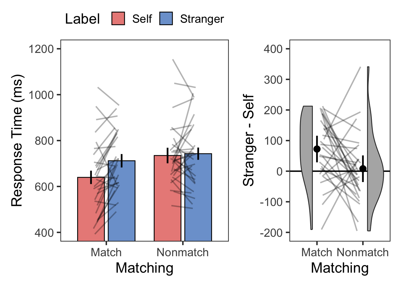
# Descriptive
dpt %>% group_by(Matching, Label) %>%
  get_summary_stats(RT, show = c("mean", "sd")) %>%
kable(digits = 0, format = "simple", caption = "Descriptive summary")| Matching | Label | variable | n | mean | sd |
|---|---|---|---|---|---|
| Match | Self | RT | 28 | 640 | 161 |
| Match | Stranger | RT | 28 | 712 | 130 |
| Nonmatch | Self | RT | 28 | 735 | 138 |
| Nonmatch | Stranger | RT | 28 | 743 | 151 |
# BF
( bf.dSpeRT <- anovaBF(RT ~ Matching*Label + SN, data = as.data.frame(dpt),
                       whichRandom = "SN", iterations = nIter, progress = FALSE) )
## Bayes factor analysis
## --------------
## [1] Matching + SN                          : 203.983  ±0.29%
## [2] Label + SN                             : 2.765072 ±0.19%
## [3] Matching + Label + SN                  : 946.8884 ±0.39%
## [4] Matching + Label + Matching:Label + SN : 1889.554 ±0.95%
##
## Against denominator:
##   RT ~ SN
## ---
## Bayes factor type: BFlinearModel, JZS
# plot(bf.dSpeRT)

# ANOVA
cbind(
  anova_test(
    data = dpt, dv = RT, wid = SN,
    within = c(Matching, Label),
    effect.size = "pes") %>%
    get_anova_table() ,
  tibble(BF10 = c( exp((bf.dSpeRT[3]/bf.dSpeRT[2])@bayesFactor$bf),
                   exp((bf.dSpeRT[3]/bf.dSpeRT[1])@bayesFactor$bf),
                   exp((bf.dSpeRT[4]/bf.dSpeRT[3])@bayesFactor$bf) ),
         BF01 = c( exp((bf.dSpeRT[2]/bf.dSpeRT[3])@bayesFactor$bf),
                   exp((bf.dSpeRT[1]/bf.dSpeRT[3])@bayesFactor$bf),
                   exp((bf.dSpeRT[3]/bf.dSpeRT[4])@bayesFactor$bf) ))) %>%
kable(digits = c(0,0,0,3,4,0,3,3,3), format = "simple", caption = "ANOVA")| Effect | DFn | DFd | F | p | p<.05 | pes | BF10 | BF01 |
|---|---|---|---|---|---|---|---|---|
| Matching | 1 | 27 | 18.699 | 0.0002 | * | 0.409 | 342.446 | 0.003 |
| Label | 1 | 27 | 8.181 | 0.0080 | * | 0.233 | 4.642 | 0.215 |
| Matching:Label | 1 | 27 | 4.605 | 0.0410 | * | 0.146 | 1.996 | 0.501 |
# Post-hoc
dgT <- 3
dgP <- 3
dgM <- 0
dgC <- 0
dgD <- 3
cbind(dpt %>%
        group_by(Matching) %>%
        t_test(RT ~ Label, ref.group = "Stranger",
               paired = TRUE, detailed = TRUE) %>%
        adjust_pvalue(method = "bonferroni") %>%
        add_significance("p.adj") %>%
        unite("Comparison", group1:group2, sep = " > ") %>%
        mutate("95% CI" = paste0("[", round(conf.low, digits = dgC), ", ",
                                 round(conf.high, digits = dgC), "]")) %>%
        rename('T' = statistic, M = estimate) %>%
        select(Matching, Comparison, 'T', df, p, p.adj, p.adj.signif,
               M, '95% CI'),
      dpt %>%
        group_by(Matching) %>%
        cohens_d(RT ~ Label, paired = TRUE, ref.group = "Stranger") %>%
        select("effsize", "magnitude") %>%
        rename("Cohen's d" = effsize)) %>%
  kable(digits = c(0,0,dgT,0,dgP,dgP,0,dgM,0,dgD,0),
format = "simple", caption = "T-Test, Bonferroni Corrected")| Matching | Comparison | T | df | p | p.adj | p.adj.signif | M | 95% CI | Cohen’s d | magnitude |
|---|---|---|---|---|---|---|---|---|---|---|
| Match | Stranger > Self | 3.647 | 27 | 0.001 | 0.002 | ** | 72 | [32, 113] | 0.689 | moderate |
| Nonmatch | Stranger > Self | 0.376 | 27 | 0.710 | 1.000 | ns | 8 | [-36, 52] | 0.071 | negligible |
3.06% of RTs were removed as extreme values.
6 Correlation
We computed the correlations among self-bias scores derived from label-matching RTs in the associative learning task, and from shape-matching RTs and label-matching RTs in the working memory task.
# Associative Learning Task: Label-Matching
asc.effect <- s.rt %>%
  filter(Matching == "Match") %>%
  pivot_wider(id_cols = SN, names_from = Label, values_from = RT) %>%
  mutate(lrnLabel = Stranger - Self) %>%
  select(SN, lrnLabel)

# Working Memory Task: Shape-Matching
shape.effect <- dst %>%
  group_by(SN, Identity) %>%
  summarise(value = mean(RT)) %>%
  ungroup() %>%
  pivot_wider(id_cols = SN, names_from = Identity, values_from = value) %>%
  mutate(wmShape = Stranger - Self) %>%
  select(SN, wmShape)

# Working Memory Task: Label-Matching
tst.effect <- dpt %>%
  filter(Matching == "Match") %>%
  pivot_wider(id_cols = SN, names_from = Label, values_from = RT) %>%
  mutate(wmLabel = Stranger - Self) %>%
  select(SN, wmLabel)


self.bias <- full_join(
  full_join(asc.effect, shape.effect, by = 'SN'),
  tst.effect, by = 'SN')

self.bias %>%
  select(-SN) %>%
  pairs.panels(method = "pearson", lm = TRUE, stars = TRUE)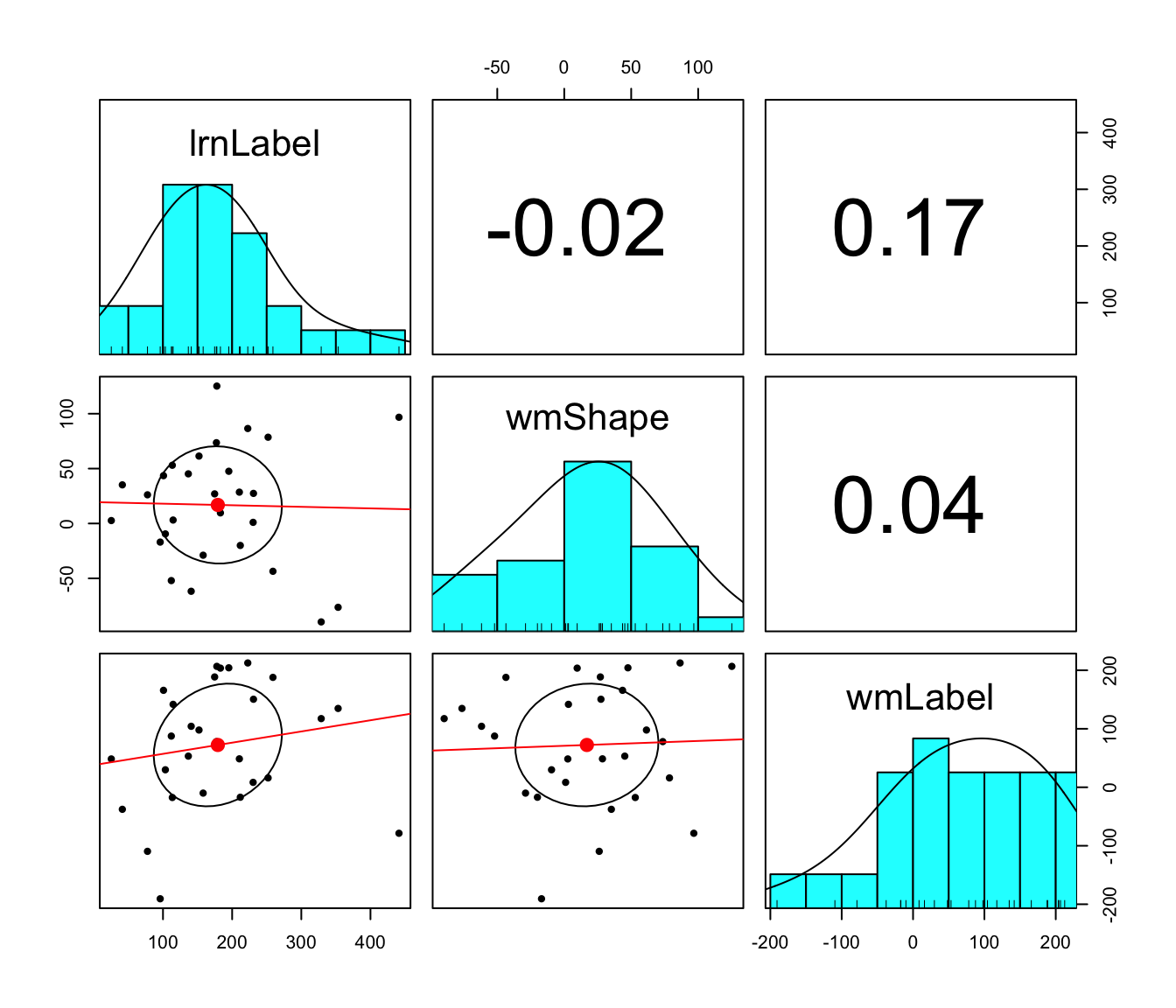
lrnLabel: label-matching self-bias in the
associative learning task
wmShape: shape-matching
self-bias in the working memory task
wmLabel:
label-matching self-bias in the working memory task
cor.mat <- self.bias  %>% select(-SN) %>% cor_mat(method = "pearson")
ctb <- cor.mat %>% cor_gather() %>% slice(c(4,7,8)) %>% rename(r = cor)
ctb <- ctb %>%
  mutate(p_bonferroni = p * 3, # Bonferroni correction
         p_bonferroni = ifelse(p_bonferroni > 1, 1, p_bonferroni))  # max = 1

# BF
( bf.corr1 <- correlationBF(y = self.bias$lrnLabel, x = self.bias$wmShape) )
## Bayes factor analysis
## --------------
## [1] Alt., r=0.333 : 0.4149212 ±0%
##
## Against denominator:
##   Null, rho = 0
## ---
## Bayes factor type: BFcorrelation, Jeffreys-beta*
( bf.corr2 <- correlationBF(y = self.bias$lrnLabel, x = self.bias$wmLabel) )
## Bayes factor analysis
## --------------
## [1] Alt., r=0.333 : 0.5625174 ±0%
##
## Against denominator:
##   Null, rho = 0
## ---
## Bayes factor type: BFcorrelation, Jeffreys-beta*
( bf.corr3 <- correlationBF(y = self.bias$wmShape, x = self.bias$wmLabel) )
## Bayes factor analysis
## --------------
## [1] Alt., r=0.333 : 0.4201243 ±0%
##
## Against denominator:
##   Null, rho = 0
## ---
## Bayes factor type: BFcorrelation, Jeffreys-beta*

ttb <- tibble(
  var1 = c('lrnLabel', 'lrnLabel', 'wmShape'),
  var2 = c('wmShape', 'wmLabel', 'wmLabel'),
  BF10 = c( exp(bf.corr1@bayesFactor$bf),
            exp(bf.corr2@bayesFactor$bf),
            exp(bf.corr3@bayesFactor$bf) ),
  BF01 = c( exp((1/bf.corr1)@bayesFactor$bf),
            exp((1/bf.corr2)@bayesFactor$bf),
            exp((1/bf.corr3)@bayesFactor$bf) ))

full_join(ctb, ttb) %>%
  kable(digits = 3, format = "simple",
        caption = "Pearson Correlation Coefficient & Bayes Factors")
## Joining with `by = join_by(var1, var2)`| var1 | var2 | r | p | p_bonferroni | BF10 | BF01 |
|---|---|---|---|---|---|---|
| lrnLabel | wmShape | -0.025 | 0.900 | 1 | 0.415 | 2.410 |
| lrnLabel | wmLabel | 0.170 | 0.390 | 1 | 0.563 | 1.778 |
| wmShape | wmLabel | 0.042 | 0.831 | 1 | 0.420 | 2.380 |
7 Session Info
sessionInfo()
## R version 4.5.1 (2025-06-13)
## Platform: aarch64-apple-darwin20
## Running under: macOS Tahoe 26.0.1
##
## Matrix products: default
## BLAS:   /Library/Frameworks/R.framework/Versions/4.5-arm64/Resources/lib/libRblas.0.dylib
## LAPACK: /Library/Frameworks/R.framework/Versions/4.5-arm64/Resources/lib/libRlapack.dylib;  LAPACK version 3.12.1
##
## locale:
## [1] en_US.UTF-8/en_US.UTF-8/en_US.UTF-8/C/en_US.UTF-8/en_US.UTF-8
##
## time zone: Asia/Seoul
## tzcode source: internal
##
## attached base packages:
## [1] stats     graphics  grDevices utils     datasets  methods   base
##
## other attached packages:
##  [1] klippy_0.0.0.9500      patchwork_1.3.2        cowplot_1.2.0
##  [4] see_0.12.0             ggpubr_0.6.1           Superpower_0.2.4.1
##  [7] BayesFactor_0.9.12-4.7 Matrix_1.7-4           coda_0.19-4.1
## [10] rstatix_0.7.2          knitr_1.50             psych_2.5.6
## [13] lubridate_1.9.4        forcats_1.0.1          stringr_1.5.2
## [16] dplyr_1.1.4            purrr_1.1.0            readr_2.1.5
## [19] tidyr_1.3.1            tibble_3.3.0           ggplot2_4.0.0
## [22] tidyverse_2.0.0
##
## loaded via a namespace (and not attached):
##  [1] tidyselect_1.2.1    viridisLite_0.4.2   farver_2.1.2
##  [4] S7_0.2.0            fastmap_1.2.0       pacman_0.5.1
##  [7] digest_0.6.37       estimability_1.5.1  timechange_0.3.0
## [10] lifecycle_1.0.4     magrittr_2.0.4      compiler_4.5.1
## [13] rlang_1.1.6         sass_0.4.10         tools_4.5.1
## [16] utf8_1.2.6          yaml_2.3.10         ggsignif_0.6.4
## [19] labeling_0.4.3      mnormt_2.1.1        plyr_1.8.9
## [22] RColorBrewer_1.1-3  abind_1.4-8         withr_3.0.2
## [25] numDeriv_2016.8-1.1 grid_4.5.1          afex_1.5-0
## [28] xtable_1.8-4        emmeans_1.11.2-8    scales_1.4.0
## [31] MASS_7.3-65         insight_1.4.2       cli_3.6.5
## [34] mvtnorm_1.3-3       crayon_1.5.3        rmarkdown_2.30
## [37] reformulas_0.4.1    generics_0.1.4      rstudioapi_0.17.1
## [40] reshape2_1.4.4      tzdb_0.5.0          minqa_1.2.8
## [43] pbapply_1.7-4       cachem_1.1.0        splines_4.5.1
## [46] assertthat_0.2.1    parallel_4.5.1      vctrs_0.6.5
## [49] boot_1.3-32         jsonlite_2.0.0      carData_3.0-5
## [52] car_3.1-3           hms_1.1.3           Formula_1.2-5
## [55] magick_2.9.0        Rmisc_1.5.1         jquerylib_0.1.4
## [58] glue_1.8.0          nloptr_2.2.1        stringi_1.8.7
## [61] gtable_0.3.6        lme4_1.1-37         lmerTest_3.1-3
## [64] pillar_1.11.1       htmltools_0.5.8.1   R6_2.6.1
## [67] Rdpack_2.6.4        evaluate_1.0.5      lattice_0.22-7
## [70] rbibutils_2.3       backports_1.5.0     broom_1.0.10
## [73] bslib_0.9.0         MatrixModels_0.5-4  Rcpp_1.1.0
## [76] nlme_3.1-168        xfun_0.53           pkgconfig_2.0.3
Copyright © 2025 CogNIPS. All rights reserved.