Experiment 2
Self-Priority Effects on Nonspatial Working Memory
Woojeong Lee & Do-Joon Yi
2025-10-01
pacman::p_load(tidyverse, psych, knitr, rstatix, BayesFactor)
pacman::p_load(ggpubr, see, cowplot)
pacman::p_load_gh("thomasp85/patchwork", 'eddjberry/mixturer')
if (!requireNamespace("Rmisc", quietly = TRUE)) install.packages("Rmisc")
if (!requireNamespace("bayestestR", quietly = TRUE)) install.packages("bayestestR")
if (!requireNamespace("magick", quietly = TRUE)) install.packages("magick")

set.seed(1234567) # for reproducibility
options(dplyr.summarise.inform=FALSE) # suppress warning in regards to regrouping
options(knitr.kable.NA = '')
options("scipen" = 100) # https://rfriend.tistory.com/224
nIter <- 1e4 # Monte Carlo simulations for error < 1%. default = 1e4
tOff <- 2.5 # RTtrimming
klippy::klippy()
deg2rad <- function(deg){deg * pi / 180}

# Plot for outlier check
single_raincloud_plot <- function(df, Y, xMin, xMax, xBy, xLab){
  df %>% ggplot(aes(x = 1, y = Y)) +
    geom_violinhalf(flip = c(1,3), width = 0.5, color = "grey70", fill = "gray70") +
    geom_point(aes(0.8, Y), size = 1.5,
               color = "grey50", fill = "grey50", alpha = .5,
               position = position_jitter(width = 0.15, height = 0)) +
    geom_boxplot(width=0.05, alpha = 0.5, outliers = FALSE) +
    scale_y_continuous(breaks=seq(xMin,xMax,by=xBy)) +
    coord_flip(ylim = c(xMin, xMax), clip = "on") +
    labs(y = xLab) +
    theme_bw(base_size = 18) +
    theme(panel.grid.major = element_blank(),
          panel.grid.minor = element_blank(),
          axis.title.y = element_blank(),
          axis.ticks.y = element_blank(),
          axis.text.y = element_blank(),
          aspect.ratio = .3)
}

## Plot for results
plotMatchLabel <- function(df, ylabel, ymin, ymax, yby,
                           OminusS, ymin2, ymax2, yby2) {
  names(df)[ncol(df)] <- "DV" # assuming DV on the last column

  df.g <- df %>%
    Rmisc::summarySEwithin(measurevar = 'DV', idvar = 'SN',
                           withinvars = c("Matching", "Label"))

  df.w <- df %>%
    unite("temp", c("Matching", "Label")) %>%
    pivot_wider(id_cols = SN, names_from = temp, values_from = DV)

  doff <- 0.03
  tmp <- runif(nrow(df.w), -doff, doff)
  spd1 <- rep(-0.14,nrow(df.w)) + tmp
  spd2 <- rep( 0.14,nrow(df.w)) + tmp

  F1 <- ggplot() +
    geom_bar(data=df.g, aes(x = Matching, y = DV, fill = Label), alpha = .6,
             stat="identity", width=0.7, linewidth=0.5, color="black",
             position=position_dodge(.8)) +
    scale_fill_manual(values=c('#DC3220', '#005AB5'),
                      labels=c("Self", "Friend")) +
    geom_segment(data=df.w, color="black", alpha = 0.3,
                 aes(x=1+spd1, y=Match_Self, xend=1+spd2, yend=Match_Friend)) +
    geom_segment(data=df.w, color="black", alpha = 0.3,
                 aes(x=2+spd1, y=Nonmatch_Self, xend=2+spd2, yend=Nonmatch_Friend)) +
    geom_linerange(data=df.g, aes(x=Matching, ymin=DV-ci, ymax=DV+ci, group=Label),
                   linewidth=1, position=position_dodge(0.8)) +
    labs(x = "Matching", y = ylabel, fill='Label ') +
    coord_cartesian(ylim = c(ymin, ymax), clip = "on") +
    scale_y_continuous(breaks=seq(ymin, ymax, by = yby)) +
    theme_bw(base_size = 18) +
    theme(legend.position="top",
          legend.spacing.x = unit(0.5, 'lines'),
          legend.margin = margin(0, 0, 0, 0),
          legend.background = element_blank(),
          panel.grid.major = element_blank(),
          panel.grid.minor = element_blank())

  if (OminusS) { # Boolean: Friend - Self
    df2.w <- df.w %>%
      mutate(Match = Match_Friend - Match_Self,
             Nonmatch = Nonmatch_Friend - Nonmatch_Self) %>%
      select(SN, Match, Nonmatch)
  } else {
    df2.w <- df.w %>%
      mutate(Match = Match_Self - Match_Friend,
             Nonmatch = Nonmatch_Self - Nonmatch_Friend) %>%
      select(SN, Match, Nonmatch)
  }

  df2 <- df2.w %>%
    pivot_longer(cols = c(Match, Nonmatch), names_to = "Matching", values_to = "SPE")

  df2.g <- df2 %>%
    mutate(Matching = factor(Matching)) %>%
    Rmisc::summarySEwithin(measurevar = "SPE", withinvars = "Matching", idvar = "SN")

  moff <- 0.1
  doff <- 0.05
  vpd <- rep(c(1-moff, 2+moff), nrow(df2)/2) # violin position dodge
  dpd <- rep(c(1+moff, 2-moff), nrow(df2)/2) + # dot position dodge
    rep(runif(nrow(df2)/2, -doff, doff), each=2)

  F2 <- cbind(df2, vpd, dpd) %>%
    ggplot(aes(x = Matching, y = SPE, group = Matching)) +
    geom_pointrange(data=df2.g, aes(x = Matching, ymin = SPE-ci, ymax = SPE+ci),
                    linewidth = 1, size = 0.5, color = "black") +
    geom_point(data=df2.g, aes(x = Matching, y = SPE),
               size=3, color = "black", show.legend = FALSE) +
    geom_hline(yintercept = 0) +
    geom_violinhalf(aes(x = vpd, y = SPE, group = Matching),
                    flip = c(1,3), width = 0.7, fill = "gray70") +
    geom_line(aes(x = dpd, y = SPE, group = SN), color = "black", alpha = 0.3) +
    labs(x = "Matching",
         y = ifelse (OminusS, # Boolean: Friend - Self
                     "Friend - Self", "Self - Friend")) +
    coord_cartesian(ylim = c(ymin2, ymax2), clip = "on") +
    scale_y_continuous(breaks=seq(ymin2, ymax2, by = yby2)) +
    theme_bw(base_size = 18) +
    theme(panel.grid.major = element_blank(),
          panel.grid.minor = element_blank())

  F1 + F2 + plot_layout(nrow = 1, widths = c(2, 1.2))
}
The current experiment was preregistered on the Open Science Framework. Participants completed an associative learning task followed by a working memory task.
1 Associative Learning Task
The task was almost identical to that in Experiment 1. Each trial presented a red or blue shape with a superimposed social label—“당신” (the Korean word for “You”) or “친구” (the Korean word for “Friend”). Participants were asked to judge whether the color of the shape matched the color that had been associated with the referent of the label (self or friend) prior to the experiment. Participants used both hands to make label-matching responses: half pressed the leftmost button (of a 9-button response box) with the left hand for “Match” and the rightmost button with the right hand for “Nonmatch,” whereas the mapping was reversed for the other half of the participants. Accuracy was computed based on all responses, and response times (RTs) were analyzed only for correct label-matching responses.
1.1 Label-Matching Accuracy
lrn <- read.csv("data/datSPE8VCS2LRN.csv", header = TRUE) %>%
  mutate(SN = factor(SN),
         Matching = factor(Matching,
                        levels = c("Match", "Nonmatch"),
                        labels = c("Match", "Nonmatch")),
         Label = factor(Label,
                        levels = c("Self", "Friend"),
                        labels = c("Self", "Friend")),
         RT = RT * 1000)
str(lrn)
## 'data.frame':    10368 obs. of  7 variables:
##  $ SN       : Factor w/ 72 levels "1","2","3","4",..: 1 1 1 1 1 1 1 1 1 1 ...
##  $ selfColor: chr  "red" "red" "red" "red" ...
##  $ Matching : Factor w/ 2 levels "Match","Nonmatch": 2 2 1 1 1 2 2 1 2 2 ...
##  $ Label    : Factor w/ 2 levels "Self","Friend": 2 1 2 2 1 1 1 2 1 2 ...
##  $ Response : chr  "Nonmatch" "Nonmatch" "Match" "Match" ...
##  $ Correct  : int  1 1 1 1 1 1 1 1 1 1 ...
##  $ RT       : num  968 841 878 1300 753 ...
length(unique(lrn$SN))
## [1] 72
table(lrn$SN)
##
##   1   2   3   4   5   6   7   8   9  10  11  12  13  14  15  16  17  18  19  20
## 144 144 144 144 144 144 144 144 144 144 144 144 144 144 144 144 144 144 144 144
##  21  22  23  24  25  26  27  28  29  30  31  32  33  34  35  36  37  38  39  40
## 144 144 144 144 144 144 144 144 144 144 144 144 144 144 144 144 144 144 144 144
##  41  42  43  44  45  46  47  48  49  50  51  52  53  54  55  56  57  58  59  60
## 144 144 144 144 144 144 144 144 144 144 144 144 144 144 144 144 144 144 144 144
##  61  62  63  64  65  66  67  68  69  70  71  72
## 144 144 144 144 144 144 144 144 144 144 144 144

# Accuracy
l.acc <- lrn %>%
  group_by(SN, Matching, Label) %>%
  summarise(Accuracy = mean(Correct)) %>%
  ungroup()

plotMatchLabel(l.acc, "Accuracy", 0.5, 1, .1, FALSE, -.2, .3, .1)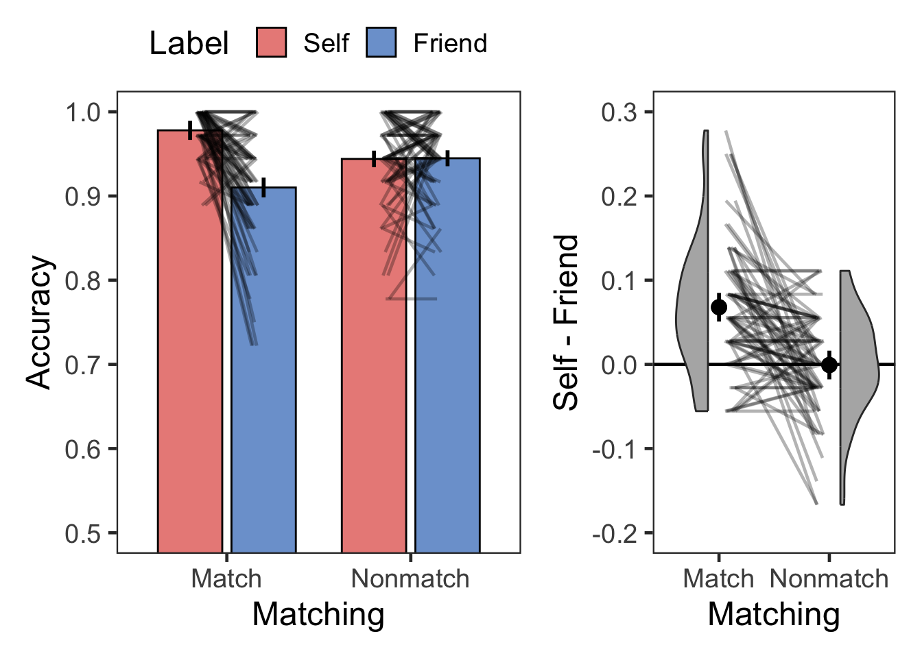
# Descriptive
l.acc %>% group_by(Matching, Label) %>%
  get_summary_stats(Accuracy, show = c("mean", "sd")) %>%
kable(digits = 2, format = "simple", caption = "Descriptive summary")| Matching | Label | variable | n | mean | sd |
|---|---|---|---|---|---|
| Match | Self | Accuracy | 72 | 0.98 | 0.03 |
| Match | Friend | Accuracy | 72 | 0.91 | 0.07 |
| Nonmatch | Self | Accuracy | 72 | 0.94 | 0.06 |
| Nonmatch | Friend | Accuracy | 72 | 0.94 | 0.05 |
bias.acc <- l.acc %>%
  filter(Matching == "Match") %>%
  pivot_wider(id_cols = "SN", names_from = "Label", values_from = "Accuracy") %>%
  mutate(selfBias = Self - Friend) %>%
  select(SN, selfBias)

bias.acc %>% get_summary_stats(selfBias, show = c("mean", "sd")) %>%
kable(digits = 2, format = "simple", caption = "Match:Self - Match:Friend")| variable | n | mean | sd |
|---|---|---|---|
| selfBias | 72 | 0.07 | 0.08 |
## Bayes factor analysis
## --------------
## [1] Alt., r=0.707 : 57953256 ±0%
##
## Against denominator:
##   Null, mu = 0
## ---
## Bayes factor type: BFoneSample, JZS
The Bayes factor indicated that the data were more than 5.795326e+07 times more likely under the alternative hypothesis than under the null hypothesis.
1.2 Label-Matching RT
range(lrn$RT[lrn$Correct==1])
## [1]  313.1731 1491.8638

lrn %>%
  filter(Correct == 1) %>%
  filter(RT < 200) %>%
  summarise(N = n())
##   N
## 1 0

lt <- lrn %>%
  filter(Correct == 1) %>%
  group_by(SN) %>%
  nest() %>%
  mutate(lbound = map(data, ~mean(.$RT)-tOff*sd(.$RT)),
         ubound = map(data, ~mean(.$RT)+tOff*sd(.$RT))) %>%
  unnest(c(lbound, ubound)) %>%
  unnest(data) %>%
  mutate(Outlier = (RT < lbound)|(RT > ubound)) %>%
  filter(Outlier == FALSE) %>%
  ungroup() %>%
  select(SN, Matching, Label,  RT)

table(lt$Matching, lt$SN)
##
##             1  2  3  4  5  6  7  8  9 10 11 12 13 14 15 16 17 18 19 20 21 22 23
##   Match    69 70 64 69 63 70 70 70 65 68 64 70 68 68 69 67 70 65 68 63 69 63 69
##   Nonmatch 72 68 63 64 62 69 71 65 64 64 67 69 69 67 67 69 67 69 70 66 68 60 69
##
##            24 25 26 27 28 29 30 31 32 33 34 35 36 37 38 39 40 41 42 43 44 45 46
##   Match    69 65 61 67 69 68 72 69 65 64 67 67 67 67 63 67 69 66 68 70 70 68 62
##   Nonmatch 69 59 67 66 68 67 68 70 68 68 71 68 67 66 70 65 67 63 67 68 67 69 56
##
##            47 48 49 50 51 52 53 54 55 56 57 58 59 60 61 62 63 64 65 66 67 68 69
##   Match    71 67 69 66 69 68 68 65 70 63 66 69 67 70 65 64 68 61 60 68 61 68 67
##   Nonmatch 71 67 67 71 67 66 69 64 69 63 65 70 64 63 70 65 67 54 65 67 64 68 69
##
##            70 71 72
##   Match    67 66 67
##   Nonmatch 66 66 65
table(lt$Label, lt$SN)
##
##           1  2  3  4  5  6  7  8  9 10 11 12 13 14 15 16 17 18 19 20 21 22 23
##   Self   72 68 68 70 62 70 72 67 67 68 66 71 70 70 65 70 69 65 70 69 69 67 71
##   Friend 69 70 59 63 63 69 69 68 62 64 65 68 67 65 71 66 68 69 68 60 68 56 67
##
##          24 25 26 27 28 29 30 31 32 33 34 35 36 37 38 39 40 41 42 43 44 45 46
##   Self   71 64 69 71 71 65 71 70 69 66 70 68 69 68 68 66 71 68 70 71 69 69 63
##   Friend 67 60 59 62 66 70 69 69 64 66 68 67 65 65 65 66 65 61 65 67 68 68 55
##
##          47 48 49 50 51 52 53 54 55 56 57 58 59 60 61 62 63 64 65 66 67 68 69
##   Self   71 69 66 69 72 69 71 68 69 65 66 72 62 64 68 67 69 63 67 69 68 70 68
##   Friend 71 65 70 68 64 65 66 61 70 61 65 67 69 69 67 62 66 52 58 66 57 66 68
##
##          70 71 72
##   Self   69 71 68
##   Friend 64 61 64
range(lt$RT)
## [1]  313.1731 1491.8638

tmp <- lt %>%
  group_by(SN, Matching, Label) %>%
  summarise(n = n()) %>%
  ungroup()
range(tmp$n) # check min & max number of trials.
## [1] 25 36
tmp %>%
  unite("Cond", Matching:Label) %>%
  pivot_wider(id_cols = SN, names_from = Cond, values_from = n) %>%
  print(n = Inf) # relatively high accuracy. seems enough number of trials.
## # A tibble: 72 × 5
##    SN    Match_Self Match_Friend Nonmatch_Self Nonmatch_Friend
##    <fct>      <int>        <int>         <int>           <int>
##  1 1             36           33            36              36
##  2 2             35           35            33              35
##  3 3             35           29            33              30
##  4 4             36           33            34              30
##  5 5             34           29            28              34
##  6 6             34           36            36              33
##  7 7             36           34            36              35
##  8 8             35           35            32              33
##  9 9             34           31            33              31
## 10 10            34           34            34              30
## 11 11            33           31            33              34
## 12 12            35           35            36              33
## 13 13            35           33            35              34
## 14 14            36           32            34              33
## 15 15            34           35            31              36
## 16 16            35           32            35              34
## 17 17            36           34            33              34
## 18 18            32           33            33              36
## 19 19            34           34            36              34
## 20 20            34           29            35              31
## 21 21            35           34            34              34
## 22 22            35           28            32              28
## 23 23            36           33            35              34
## 24 24            36           33            35              34
## 25 25            33           32            31              28
## 26 26            35           26            34              33
## 27 27            36           31            35              31
## 28 28            35           34            36              32
## 29 29            33           35            32              35
## 30 30            36           36            35              33
## 31 31            36           33            34              36
## 32 32            36           29            33              35
## 33 33            34           30            32              36
## 34 34            34           33            36              35
## 35 35            35           32            33              35
## 36 36            36           31            33              34
## 37 37            35           32            33              33
## 38 38            33           30            35              35
## 39 39            36           31            30              35
## 40 40            36           33            35              32
## 41 41            36           30            32              31
## 42 42            36           32            34              33
## 43 43            36           34            35              33
## 44 44            36           34            33              34
## 45 45            36           32            33              36
## 46 46            36           26            27              29
## 47 47            35           36            36              35
## 48 48            34           33            35              32
## 49 49            33           36            33              34
## 50 50            34           32            35              36
## 51 51            36           33            36              31
## 52 52            36           32            33              33
## 53 53            36           32            35              34
## 54 54            34           31            34              30
## 55 55            35           35            34              35
## 56 56            34           29            31              32
## 57 57            35           31            31              34
## 58 58            36           33            36              34
## 59 59            32           35            30              34
## 60 60            36           34            28              35
## 61 61            32           33            36              34
## 62 62            36           28            31              34
## 63 63            36           32            33              34
## 64 64            35           26            28              26
## 65 65            34           26            33              32
## 66 66            35           33            34              33
## 67 67            36           25            32              32
## 68 68            36           32            34              34
## 69 69            34           33            34              35
## 70 70            35           32            34              32
## 71 71            36           30            35              31
## 72 72            35           32            33              32

( pTrmd <- 100*(sum(lrn$Correct) - nrow(lt))/sum(lrn$Correct) ) # proportion of trimmed RTs
## [1] 1.777324
Among correct responses, no trials had an RT faster than 200 ms. Correct RTs exceeding ±2.5 standard deviations from the subject-specific mean were excluded from analysis, accounting for 1.78% of the data.
# RT
l.rt <- lt %>%
  group_by(SN, Matching, Label) %>%
  summarise(RT = mean(RT)) %>%
  ungroup()

plotMatchLabel(l.rt, "Response Time (ms)", 400, 1100, 200, TRUE, -100, 250, 50)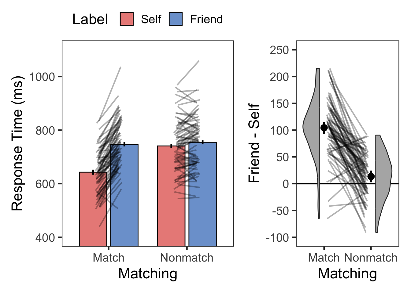
# Descriptive
l.rt %>% group_by(Matching, Label) %>%
  get_summary_stats(RT, show = c("mean", "sd")) %>%
kable(digits = 0, format = "simple", caption = "Descriptive summary")| Matching | Label | variable | n | mean | sd |
|---|---|---|---|---|---|
| Match | Self | RT | 72 | 643 | 82 |
| Match | Friend | RT | 72 | 747 | 91 |
| Nonmatch | Self | RT | 72 | 741 | 97 |
| Nonmatch | Friend | RT | 72 | 754 | 102 |
bias.rt <- l.rt %>%
  filter(Matching == "Match") %>%
  pivot_wider(id_cols = "SN", names_from = "Label", values_from = "RT") %>%
  mutate(selfBias = Friend - Self) %>%
  select(SN, selfBias)

bias.rt %>% get_summary_stats(selfBias, show = c("mean", "sd")) %>%
kable(digits = 2, format = "simple", caption = "Match:Friend - Match:Self")| variable | n | mean | sd |
|---|---|---|---|
| selfBias | 72 | 104.39 | 55.95 |
## Bayes factor analysis
## --------------
## [1] Alt., r=0.707 : 7063649214112056999936 ±0%
##
## Against denominator:
##   Null, mu = 0
## ---
## Bayes factor type: BFoneSample, JZS
The Bayes factor indicated that the data were more than 7.063649e+21 times more likely under the alternative hypothesis than under the null hypothesis.
2 Working Memory Task
At the beginning of each trial, a blue and a red object appeared on the screen. Participants were required to briefly hold the colors and shapes of the objects in working memory. After a 2-second delay, a social label and a color wheel appeared along with a mouse cursor. Participants were asked to identify the shape of the object that had been presented in the color associated with the referent of the label.
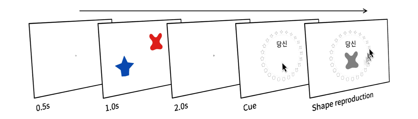
We measured the memory error (in a whole number from -179° to 180°) by calculating the angular deviation of a response from the ‘target’ shape cued by a label in each trial. As in Yin & Chen (2024), WM precision is then calculated separately for each participant and condition as the reciprocal of the standard deviation of memory errors across trials. The estimation of WM precision is based on the formula described in prior works (Bays et al., 2009).
2.1 Precision
2.1.1 Descriptive Stats
tst <- read.csv("data/datSPE8VCS2TST.csv") %>%
  mutate(SN = factor(SN),
         Label = factor(Label,
                        levels = c("Self", "Friend"),
                        labels = c("Self", "Friend"))) %>%
  mutate(ErrorRad = deg2rad(Error))
str(tst)
## 'data.frame':    10368 obs. of  18 variables:
##  $ SN        : Factor w/ 72 levels "1","2","3","4",..: 1 1 1 1 1 1 1 1 1 1 ...
##  $ selfColor : chr  "red" "red" "red" "red" ...
##  $ Trial     : int  1 2 3 4 5 6 7 8 9 10 ...
##  $ selfSide  : chr  "left" "left" "right" "left" ...
##  $ otherSide : chr  "right" "right" "left" "right" ...
##  $ selfID    : int  314 218 4 245 87 65 96 291 243 274 ...
##  $ otherID   : int  20 107 184 332 153 221 360 358 33 201 ...
##  $ Label     : Factor w/ 2 levels "Self","Friend": 1 2 2 1 1 2 2 2 2 1 ...
##  $ TrgSide   : int  1 2 1 1 2 2 2 1 2 1 ...
##  $ TrgColor  : chr  "red" "blue" "blue" "red" ...
##  $ wheelShift: int  339 322 55 215 310 281 103 275 352 133 ...
##  $ TrgLoc    : int  293 69 239 100 37 142 103 273 25 47 ...
##  $ TrgID     : int  314 107 184 245 87 221 360 358 33 274 ...
##  $ RspLoc    : int  299 65 240 112 46 139 93 264 13 71 ...
##  $ RspID     : int  320 103 185 257 96 218 350 349 21 298 ...
##  $ Error     : int  6 -4 1 12 9 -3 -10 -9 -12 24 ...
##  $ RT        : num  4.9 6.54 6.27 6.65 7.06 ...
##  $ ErrorRad  : num  0.1047 -0.0698 0.0175 0.2094 0.1571 ...
length(unique(tst$SN))
## [1] 72
table(tst$selfColor, tst$SN)
##
##          1   2   3   4   5   6   7   8   9  10  11  12  13  14  15  16  17  18
##   blue   0 144   0 144   0 144   0 144   0 144   0 144   0 144   0 144   0 144
##   red  144   0 144   0 144   0 144   0 144   0 144   0 144   0 144   0 144   0
##
##         19  20  21  22  23  24  25  26  27  28  29  30  31  32  33  34  35  36
##   blue   0 144   0 144   0 144   0 144   0 144   0 144   0 144   0 144   0 144
##   red  144   0 144   0 144   0 144   0 144   0 144   0 144   0 144   0 144   0
##
##         37  38  39  40  41  42  43  44  45  46  47  48  49  50  51  52  53  54
##   blue   0 144   0 144   0 144   0 144   0 144   0 144   0 144   0 144   0 144
##   red  144   0 144   0 144   0 144   0 144   0 144   0 144   0 144   0 144   0
##
##         55  56  57  58  59  60  61  62  63  64  65  66  67  68  69  70  71  72
##   blue   0 144   0 144   0 144   0 144   0 144   0 144   0 144   0 144   0 144
##   red  144   0 144   0 144   0 144   0 144   0 144   0 144   0 144   0 144   0

range(tst$Error)
## [1] -179  180
range(deg2rad(tst$Error))
## [1] -3.124139  3.141593

headTail(tst)
##         SN selfColor Trial selfSide otherSide selfID otherID  Label TrgSide
## 1        1       red     1     left     right    314      20   Self       1
## 2        1       red     2     left     right    218     107 Friend       2
## 3        1       red     3    right      left      4     184 Friend       1
## 4        1       red     4     left     right    245     332   Self       1
## ...   <NA>      <NA>   ...     <NA>      <NA>    ...     ...   <NA>     ...
## 10365   72      blue   141    right      left    110      74 Friend       1
## 10366   72      blue   142    right      left    177      52   Self       2
## 10367   72      blue   143    right      left    281     143   Self       2
## 10368   72      blue   144     left     right     86     222   Self       1
##       TrgColor wheelShift TrgLoc TrgID RspLoc RspID Error   RT ErrorRad
## 1          red        339    293   314    299   320     6  4.9      0.1
## 2         blue        322     69   107     65   103    -4 6.54    -0.07
## 3         blue         55    239   184    240   185     1 6.27     0.02
## 4          red        215    100   245    112   257    12 6.65     0.21
## ...       <NA>        ...    ...   ...    ...   ...   ...  ...      ...
## 10365      red         33    107    74    105    72    -2 3.88    -0.03
## 10366     blue        318    135   177    155   197    20 5.46     0.35
## 10367     blue        174     95   281     99   285     4  7.5     0.07
## 10368     blue         11     97    86     98    87     1 3.99     0.02

# # Error는 아래 두 가지 방식으로 변인을 조합하여 재현할 수 있다.
# tst %>% mutate(tmp1 = (RspID - TrgID) %% 360,
#                tmp2 = ifelse(tmp1 > 180, tmp1-360, tmp1),
#                tmp3 = 1- (Error==tmp2)) %>%
#   summarise(sumError = sum(tmp3))
#
# tst %>% mutate(tmp1 = (RspLoc - TrgLoc) %% 360,
#                tmp2 = ifelse(tmp1 > 180, tmp1-360, tmp1),
#                tmp3 = 1- (Error==tmp2)) %>%
#   summarise(sumError = sum(tmp3))


# Outlier Detection on precision

F3 <- tst %>% select(Label, ErrorRad) %>%
  ggplot() +
  geom_histogram(mapping = aes(x = ErrorRad,
                               y = after_stat(density),
                               fill = Label),
                 position = 'identity', binwidth = pi/18, alpha = 0.4) +
  geom_density(mapping = aes(x = ErrorRad, color = Label),
               alpha = 0.5, linewidth = 0.5) +
  scale_x_continuous(breaks = c(-pi, -pi/2, 0, pi/2, pi),
                     label = c(expression(-pi), expression(-pi/2),
                               0, expression(pi/2), expression(pi))) +
  labs(x = "Memory Error (rad)", y = "Density") +
  # facet_grid(. ~ Label) +
  scale_fill_manual(values=c("#DC3220", "#005AB5")) +
  scale_color_manual(values=c("#DC3220", "#005AB5")) +
  theme_bw(base_size = 18) +
  theme(legend.position="top",
        legend.spacing.x = unit(0.5, 'lines'),
        legend.margin = margin(0, 0, 0, 0),
        legend.background = element_blank(),
        strip.background = element_blank(),
        panel.grid.major = element_blank(),
        panel.grid.minor = element_blank())

t1 <- tst %>%
  group_by(SN, Label) %>%
  group_modify( ~ bays_2009_error(.$ErrorRad)) %>%
  ungroup() %>%
  rename(Precision = precision)
headTail(t1)
##     SN  Label Precision  bias
## 1    1   Self      2.64     0
## 2    1 Friend      1.05  0.05
## 3    2   Self      2.34 -0.05
## 4    2 Friend      2.43 -0.01
## 5 <NA>   <NA>       ...   ...
## 6   71   Self      2.04  0.13
## 7   71 Friend      2.32  0.14
## 8   72   Self      1.46   0.1
## 9   72 Friend      2.07  0.03
t1 %>% print(n = Inf)
## # A tibble: 144 × 4
##     SN    Label  Precision       bias
##     <fct> <fct>      <dbl>      <dbl>
##   1 1     Self       2.64  -0.00418
##   2 1     Friend     1.05   0.0525
##   3 2     Self       2.34  -0.0461
##   4 2     Friend     2.43  -0.00570
##   5 3     Self       1.34   0.0500
##   6 3     Friend     1.61   0.000374
##   7 4     Self       2.10  -0.0371
##   8 4     Friend     1.75  -0.00726
##   9 5     Self       1.29   0.0683
##  10 5     Friend     1.43   0.0195
##  11 6     Self       3.16  -0.00786
##  12 6     Friend     2.65   0.0660
##  13 7     Self       1.62   0.0111
##  14 7     Friend     1.49  -0.00115
##  15 8     Self       1.93  -0.0178
##  16 8     Friend     1.10  -0.0117
##  17 9     Self       1.26   0.00847
##  18 9     Friend     1.74  -0.0283
##  19 10    Self       1.81   0.0390
##  20 10    Friend     1.23   0.0668
##  21 11    Self       1.30   0.0596
##  22 11    Friend     1.14   0.0569
##  23 12    Self       0.876  0.0738
##  24 12    Friend     1.66   0.115
##  25 13    Self       1.68   0.0485
##  26 13    Friend     1.44  -0.000924
##  27 14    Self       0.984  0.0382
##  28 14    Friend     0.770  0.131
##  29 15    Self       1.53   0.0461
##  30 15    Friend     3.00  -0.0445
##  31 16    Self       1.03   0.000253
##  32 16    Friend     1.14  -0.0265
##  33 17    Self       3.02  -0.0213
##  34 17    Friend     2.70   0.0000167
##  35 18    Self       2.50   0.0320
##  36 18    Friend     5.03   0.0359
##  37 19    Self       2.59   0.0456
##  38 19    Friend     2.24  -0.0136
##  39 20    Self       1.52   0.0148
##  40 20    Friend     2.37   0.0367
##  41 21    Self       1.66  -0.0353
##  42 21    Friend     1.32  -0.0808
##  43 22    Self       1.81   0.0764
##  44 22    Friend     1.50   0.0459
##  45 23    Self       2.60   0.0175
##  46 23    Friend     2.72   0.0668
##  47 24    Self       1.97   0.0224
##  48 24    Friend     1.69  -0.00311
##  49 25    Self       2.11   0.0487
##  50 25    Friend     0.956  0.121
##  51 26    Self       1.41   0.0332
##  52 26    Friend     0.811  0.0847
##  53 27    Self       2.57   0.0571
##  54 27    Friend     2.05  -0.0837
##  55 28    Self       0.644 -0.153
##  56 28    Friend     0.801  0.0801
##  57 29    Self       2.15   0.000375
##  58 29    Friend     3.60   0.0341
##  59 30    Self       2.31  -0.0228
##  60 30    Friend     3.71   0.00463
##  61 31    Self       1.75   0.0469
##  62 31    Friend     1.55  -0.0370
##  63 32    Self       2.17   0.0406
##  64 32    Friend     3.07   0.0739
##  65 33    Self       1.84   0.0277
##  66 33    Friend     3.75   0.00995
##  67 34    Self       2.07  -0.0240
##  68 34    Friend     2.01  -0.0918
##  69 35    Self       1.75   0.0165
##  70 35    Friend     0.982  0.155
##  71 36    Self       1.35  -0.0794
##  72 36    Friend     1.36  -0.0318
##  73 37    Self       2.11  -0.00773
##  74 37    Friend     3.07  -0.0387
##  75 38    Self       2.07   0.0203
##  76 38    Friend     2.46  -0.0574
##  77 39    Self       1.98  -0.0196
##  78 39    Friend     2.31  -0.0616
##  79 40    Self       2.69   0.00118
##  80 40    Friend     3.11  -0.0170
##  81 41    Self       2.73  -0.0415
##  82 41    Friend     2.25  -0.0236
##  83 42    Self       1.98   0.0980
##  84 42    Friend     1.72   0.0795
##  85 43    Self       1.12   0.0505
##  86 43    Friend     1.77   0.0938
##  87 44    Self       1.53  -0.0519
##  88 44    Friend     2.29   0.00571
##  89 45    Self       1.44  -0.0325
##  90 45    Friend     1.79  -0.0348
##  91 46    Self       0.950 -0.0513
##  92 46    Friend     1.87   0.00413
##  93 47    Self       1.69   0.0274
##  94 47    Friend     1.20   0.0896
##  95 48    Self       1.83   0.0571
##  96 48    Friend     1.94   0.00955
##  97 49    Self       0.922 -0.0153
##  98 49    Friend     1.44   0.0523
##  99 50    Self       1.50   0.00483
## 100 50    Friend     1.77  -0.154
## 101 51    Self       2.46   0.0605
## 102 51    Friend     2.16   0.0387
## 103 52    Self       1.97  -0.0154
## 104 52    Friend     2.06  -0.0516
## 105 53    Self       2.72  -0.0192
## 106 53    Friend     1.72   0.0373
## 107 54    Self       2.21   0.0960
## 108 54    Friend     3.23   0.0672
## 109 55    Self       2.14  -0.0843
## 110 55    Friend     1.70  -0.0504
## 111 56    Self       2.00   0.0162
## 112 56    Friend     1.24   0.000818
## 113 57    Self       1.27   0.0364
## 114 57    Friend     1.32   0.0282
## 115 58    Self       4.45  -0.0216
## 116 58    Friend     3.93   0.0175
## 117 59    Self       1.64   0.0310
## 118 59    Friend     1.80   0.0470
## 119 60    Self       1.54   0.0161
## 120 60    Friend     1.63   0.0735
## 121 61    Self       1.04   0.0172
## 122 61    Friend     0.836 -0.00979
## 123 62    Self       1.60   0.0454
## 124 62    Friend     1.67  -0.0297
## 125 63    Self       2.28   0.0550
## 126 63    Friend     3.22   0.0268
## 127 64    Self       1.24   0.0596
## 128 64    Friend     0.672 -0.0949
## 129 65    Self       1.63   0.0314
## 130 65    Friend     2.00   0.0836
## 131 66    Self       2.40   0.00217
## 132 66    Friend     1.75  -0.0496
## 133 67    Self       0.678  0.0531
## 134 67    Friend     0.764 -0.0974
## 135 68    Self       2.20  -0.0134
## 136 68    Friend     2.23  -0.0567
## 137 69    Self       1.56   0.0392
## 138 69    Friend     1.66   0.0303
## 139 70    Self       1.53   0.0565
## 140 70    Friend     1.97   0.0126
## 141 71    Self       2.04   0.134
## 142 71    Friend     2.32   0.140
## 143 72    Self       1.46   0.104
## 144 72    Friend     2.07   0.0303

t1.g <- t1 %>%
  Rmisc::summarySEwithin(measurevar = 'Precision', idvar = 'SN',
                         withinvars = "Label")
t1.w <- t1 %>%
  pivot_wider(id_cols = SN, names_from = Label, values_from = Precision)

pd <- rep(c(1.1, 1.9), 72)
F4 <- ggplot() +
  geom_bar(data=t1.g, aes(x = Label, y = Precision, fill = Label), alpha = .6,
           stat="identity", width=0.7, linewidth=0.5, color="black") +
  # geom_point(data=cbind(t1, pd), aes(x = pd, y = Precision, group = Label),
  #            color="gray80", alpha=0.5, size=1.8) +
  geom_segment(data=t1.w, color="black", alpha=0.3,
               aes(x=1+.1, y=Self, xend=2-.1, yend=Friend)) +
  geom_linerange(data=t1.g, aes(x=Label, ymin=Precision-ci, ymax=Precision+ci, group=Label),
                 linewidth=1) +
  # geom_point(data=t1.g, aes(x = Label, y = Precision),
  #            size=3, color = "black", show.legend = FALSE) +
  scale_fill_manual(values=c('#DC3220', '#005AB5'),
                    labels=c("Self", "Friend")) +
  labs(x = "Label", y = expression("Precision (" * rad^{-1} * ")")) +
  coord_cartesian(ylim = c(0, 5), clip = "on") +
  scale_y_continuous(breaks=seq(0, 5, by = 1)) +
  theme_bw(base_size = 18) +
  theme(legend.position= "none",
        panel.grid.major = element_blank(),
        panel.grid.minor = element_blank())
# , position = position_nudge(x = .1, y = 0)

F3 + F4 + plot_layout(nrow = 1, widths = c(1, 1))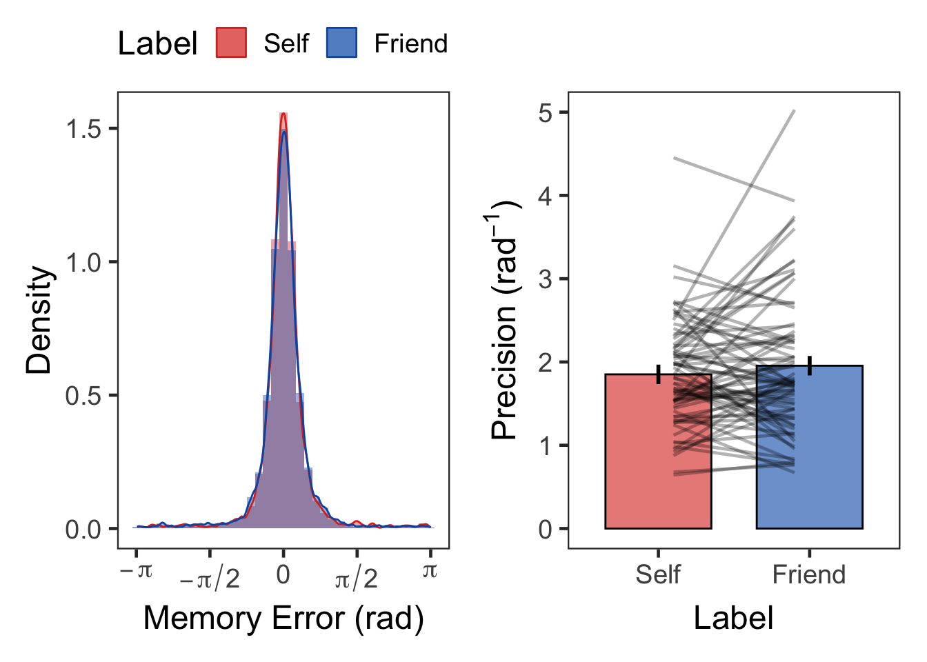
# Descriptive
t1 %>% group_by(Label) %>%
  get_summary_stats(Precision, show = c("mean", "sd")) %>%
kable(digits = 2, format = "simple", caption = "Descriptive summary")| Label | variable | n | mean | sd |
|---|---|---|---|---|
| Self | Precision | 72 | 1.85 | 0.64 |
| Friend | Precision | 72 | 1.96 | 0.85 |
2.1.2 Bayes Factor
## Bayes factor analysis
## --------------
## [1] Alt., r=0.707 0<d<Inf    : 0.06099351 ±0%
## [2] Alt., r=0.707 !(0<d<Inf) : 0.4880014  ±0%
##
## Against denominator:
##   Null, mu = 0
## ---
## Bayes factor type: BFoneSample, JZS## Bayes factor analysis
## --------------
## [1] Null, mu=0 : 16.39519 ±0%
##
## Against denominator:
## Alternative, r = 0.707, mu =/= 0 0<d<Inf
## ---
## Bayes factor type: BFoneSample, JZSThe Bayes factor indicated that the data were more than 16.395187 times more likely under the null hypothesis than under the directional alaternative hypothesis.
plot(bayestestR::bayesfactor_models(bf1[1])) +
  scale_fill_pizza() +
  scale_fill_manual(values=c('#E69F00', '#56B4E9')) +
  theme(text = element_text(size = 18))
## Scale for fill is already present.
## Adding another scale for fill, which will replace the existing scale.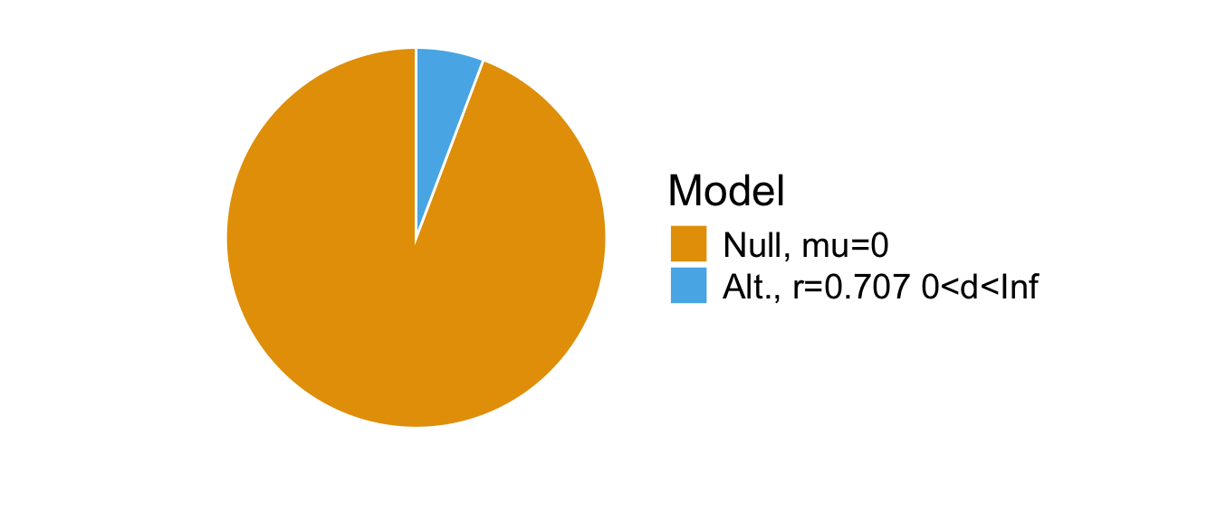
3 Correlation
Self-bias were computed separately for label-matching RTs in the associative learning task and for precision in the working memory task.
For label-matching RTs, self-bias was defined as the difference between the self and friend conditions on match trials, following prior research (Yin et al., 2019). For WM precision, it was defined as the difference between the self and friend conditions.
A Pearson correlation was then calculated between the two self-bias measures.
lrn.matching <- l.rt %>%
  filter(Matching == "Match") %>%
  pivot_wider(id_cols = SN, names_from = Label, values_from = RT) %>%
  mutate(lrnLabel = Friend - Self) %>%
  select(SN, lrnLabel)

tst.precision <- t1 %>%
  pivot_wider(id_cols = SN, names_from = Label, values_from = Precision) %>%
  mutate(wmShape = Self - Friend) %>%
  select(SN, wmShape)

spe.effects <- full_join(
  lrn.matching, tst.precision, by = 'SN')
# spe.effects %>% print(n = Inf)
# https://cran.r-project.org/web/packages/BayesFactor/vignettes/manual.html#lincor
bf2 <- correlationBF(x = spe.effects$lrnLabel,
y = spe.effects$wmShape, rscale = 0.707)
bf2## Bayes factor analysis
## --------------
## [1] Alt., r=0.707 : 0.8554105 ±0%
##
## Against denominator:
## Null, rho = 0
## ---
## Bayes factor type: BFcorrelation, Jeffreys-beta*The Bayes factor indicated that the data were more than 1.1690293 times more likely under the null hypothesis than under the directional alaternative hypothesis.
# cor.test(x = spe.effects$lrnLabel, y = spe.effects$wmShape)
spe.effects %>% cor_test(lrnLabel, wmShape) %>%
  mutate("95% CI" = paste0("[", round(conf.low, digits = 3), ", ",
                                 round(conf.high, digits = 3), "]")) %>%
  select(var1, var2, method, cor, '95% CI', statistic, p) %>%
  rename(Variable1 = var1, Variable2 = var2, r = cor) %>%
kable(digits = 3, format = "simple", align = "llrrrrr", caption = "Correlation")| Variable1 | Variable2 | method | r | 95% CI | statistic | p |
|---|---|---|---|---|---|---|
| lrnLabel | wmShape | Pearson | 0.21 | [-0.02, 0.423] | 1.821 | 0.073 |
bf2 %>% bayestestR::describe_posterior()
## Summary of Posterior Distribution
##
## Parameter | Median |        95% CI |     pd |          ROPE | % in ROPE |    BF |               Prior
## -----------------------------------------------------------------------------------------------------
## rho       |   0.20 | [-0.02, 0.40] | 96.20% | [-0.05, 0.05] |     7.16% | 0.855 | Beta (1.41 +- 1.41)

C1 <- ggplot(spe.effects, aes(x=lrnLabel, y=wmShape)) +
  geom_point(size = 3, alpha = 0.5) +
  geom_smooth(method=lm, formula = y ~ x) +
  labs(x = expression(paste("Self-Bias" [" AL Task"])),
       y = expression(paste("Self-Bias" [" WM Task"]))) +
  theme_bw(base_size = 18) +
  theme(panel.grid.major = element_blank(),
        panel.grid.minor = element_blank(),
        aspect.ratio = 1) +
  annotate(geom = "text", x = 50, y = -2.2, hjust = 0, size = 5,
           label = "paste(italic(r), \" = .21, \", italic(p), \" = .07\")",
           parse = TRUE)
C2 <- plot(bayestestR::bayesfactor_models(bf2)) +
  scale_fill_pizza() +
  scale_fill_manual(values=c('#E69F00', '#56B4E9')) +
  theme(text = element_text(size = 18))
## Scale for fill is already present.
## Adding another scale for fill, which will replace the existing scale.

C1 + C2 + plot_layout(nrow = 1, widths = c(1.5, 1))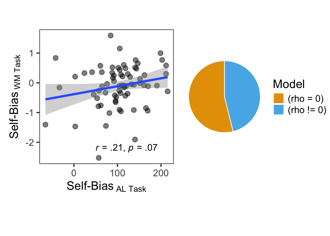
4 Session Info
sessionInfo()
## R version 4.5.1 (2025-06-13)
## Platform: aarch64-apple-darwin20
## Running under: macOS Tahoe 26.0.1
##
## Matrix products: default
## BLAS:   /Library/Frameworks/R.framework/Versions/4.5-arm64/Resources/lib/libRblas.0.dylib
## LAPACK: /Library/Frameworks/R.framework/Versions/4.5-arm64/Resources/lib/libRlapack.dylib;  LAPACK version 3.12.1
##
## locale:
## [1] en_US.UTF-8/en_US.UTF-8/en_US.UTF-8/C/en_US.UTF-8/en_US.UTF-8
##
## time zone: Asia/Seoul
## tzcode source: internal
##
## attached base packages:
## [1] stats     graphics  grDevices utils     datasets  methods   base
##
## other attached packages:
##  [1] mixturer_0.1.0         patchwork_1.3.2        cowplot_1.2.0
##  [4] see_0.12.0             ggpubr_0.6.1           BayesFactor_0.9.12-4.7
##  [7] Matrix_1.7-4           coda_0.19-4.1          rstatix_0.7.2
## [10] knitr_1.50             psych_2.5.6            lubridate_1.9.4
## [13] forcats_1.0.1          stringr_1.5.2          dplyr_1.1.4
## [16] purrr_1.1.0            readr_2.1.5            tidyr_1.3.1
## [19] tibble_3.3.0           ggplot2_4.0.0          tidyverse_2.0.0
##
## loaded via a namespace (and not attached):
##  [1] gtable_0.3.6       bayestestR_0.17.0  xfun_0.53          bslib_0.9.0
##  [5] caTools_1.18.3     insight_1.4.2      lattice_0.22-7     tzdb_0.5.0
##  [9] bitops_1.0-9       vctrs_0.6.5        tools_4.5.1        generics_0.1.4
## [13] datawizard_1.2.0   parallel_4.5.1     klippy_0.0.0.9500  pacman_0.5.1
## [17] pkgconfig_2.0.3    RColorBrewer_1.1-3 S7_0.2.0           assertthat_0.2.1
## [21] lifecycle_1.0.4    compiler_4.5.1     farver_2.1.2       MatrixModels_0.5-4
## [25] mnormt_2.1.1       carData_3.0-5      htmltools_0.5.8.1  sass_0.4.10
## [29] yaml_2.3.10        Formula_1.2-5      pillar_1.11.1      car_3.1-3
## [33] jquerylib_0.1.4    cachem_1.1.0       magick_2.9.0       abind_1.4-8
## [37] nlme_3.1-168       tidyselect_1.2.1   digest_0.6.37      mvtnorm_1.3-3
## [41] stringi_1.8.7      splines_4.5.1      labeling_0.4.3     fastmap_1.2.0
## [45] grid_4.5.1         cli_3.6.5          magrittr_2.0.4     Rmisc_1.5.1
## [49] utf8_1.2.6         broom_1.0.10       withr_3.0.2        scales_1.4.0
## [53] backports_1.5.0    timechange_0.3.0   rmarkdown_2.30     ggsignif_0.6.4
## [57] hms_1.1.3          pbapply_1.7-4      evaluate_1.0.5     mgcv_1.9-3
## [61] rlang_1.1.6        Rcpp_1.1.0         glue_1.8.0         rstudioapi_0.17.1
## [65] jsonlite_2.0.0     plyr_1.8.9         R6_2.6.1
Copyright © 2025 CogNIPS. All rights reserved.