Experiment 2
Words vs. Pseudowords (between-participants design)
Hongmi Lee, Kyungmi Kim, Do-Joon Yi
2019-04-03
set.seed(12345) # for reproducibility
options(knitr.kable.NA = '')

# Some packages need to be loaded. We use `pacman` as a package manager, which takes care of the other packages.
if (!require("pacman", quietly = TRUE)) install.packages("pacman")
if (!require("Rmisc", quietly = TRUE)) install.packages("Rmisc") # Never load it directly.
pacman::p_load(tidyverse, knitr, car, afex, emmeans, parallel, ordinal,
               ggbeeswarm, RVAideMemoire)
pacman::p_load_gh("crsh/papaja", "thomasp85/patchwork", "RLesur/klippy")

klippy::klippy()
1 Item Repetition Phase
Thirty participants were recruited. Half of the participants were exposed to 24 words while the other half were exposed to 24 pseudowords (pre-experimental stimulus familiarity as a between-participants factor).1 Each item was repeated eight times, resulting in 192 trials. Participants made a preference judgment (like/dislike) for each item.
P1 <- read.csv("data/data_FamSM_Exp2_Word_REP.csv", header = T)
P1$Familiarity = factor(P1$Familiarity, levels=c(1,2), labels=c("Words","Pseudowords"))
P1$Pref <- ifelse(P1$Resp==1,1,0)

glimpse(P1, width=70)
## Observations: 5,760
## Variables: 9
## $ SID         <int> 1, 1, 1, 1, 1, 1, 1, 1, 1, 1, 1, 1, 1, 1, 1, 1,…
## $ Familiarity <fct> Words, Words, Words, Words, Words, Words, Words…
## $ RepTime     <int> 1, 1, 1, 1, 1, 1, 1, 1, 1, 1, 1, 1, 1, 1, 1, 1,…
## $ Trial       <int> 1, 2, 3, 4, 5, 6, 7, 8, 9, 10, 11, 12, 13, 14, …
## $ Resp        <int> 2, 1, 1, 2, 2, 1, 1, 1, 1, 2, 2, 1, 1, 1, 1, 2,…
## $ Corr        <int> 1, 1, 1, 1, 1, 1, 1, 1, 1, 1, 1, 1, 1, 1, 1, 1,…
## $ RT          <dbl> 880.96, 868.35, 620.83, 669.82, 1006.57, 551.29…
## $ ImgName     <fct> wordin2_11.png, wordex2_9.png, wordex2_1.png, w…
## $ Pref        <dbl> 0, 1, 1, 0, 0, 1, 1, 1, 1, 0, 0, 1, 1, 1, 1, 0,…
# 1. SID: participant ID
# 2. Familiarity: pre-experimental familiarity. 1 = words, 2 = pseudowords
# 3. RepTime: number of repetition, 1~8
# 4. Trial: 1~24
# 5. Resp: preference judgment, 1 = like, 2 = dislike, 0 = no response
# 6. Corr: correctness, 1 = response, 0 = no response
# 7. RT: reaction times in ms.
# 8. ImgName: name of stimuli
# 9. Pref: preference, 0 = dislike (treating no response as 'dislike'), 1 = like

table(P1$Familiarity, P1$SID)
##
##                 1   2   3   4   5   6   7   8   9  10  11  12  13  14  15
##   Words       192 192 192 192 192 192 192 192 192 192 192 192 192 192 192
##   Pseudowords   0   0   0   0   0   0   0   0   0   0   0   0   0   0   0
##
##                16  17  18  19  20  21  22  23  24  25  26  27  28  29  30
##   Words         0   0   0   0   0   0   0   0   0   0   0   0   0   0   0
##   Pseudowords 192 192 192 192 192 192 192 192 192 192 192 192 192 192 192

1 - mean(P1$Corr)
## [1] 0.02083333
Participants did not make responses in 2.08% of trials.
1.1 Preference
We calculated the mean and s.d. of individual participants’ preference scores (probability of ‘Like’ responses) in each condition. Participants showed greater preference for words than for pseudowords. In the following plot, red points and error bars represent the means and 95% CIs.
# phase 1, subject-level, long-format
P1slong <- P1 %>% group_by(SID, Familiarity) %>%
  summarise(Preference = mean(Pref)) %>%
  ungroup()

# summary table
P1slong %>% group_by(Familiarity) %>%
  summarise(M = mean(Preference), SD = sd(Preference)) %>%
  ungroup() %>%
kable()| Familiarity | M | SD |
|---|---|---|
| Words | 0.6218750 | 0.1588914 |
| Pseudowords | 0.4270833 | 0.1667364 |
# group level, needed for printing & geom_pointrange
# Rmisc must be called indirectly due to incompatibility between plyr and dplyr.
P1g <- Rmisc::summarySE(data = P1slong, measurevar = "Preference", groupvars = "Familiarity")

ggplot(P1slong, aes(x=Familiarity, y=Preference)) +
  geom_violin(width = 0.5, trim=TRUE) +
  ggbeeswarm::geom_quasirandom(color = "blue", size = 3, alpha = 0.2, width = 0.2) +
  geom_pointrange(P1g, inherit.aes=FALSE,
                  mapping=aes(x = Familiarity, y=Preference,
                              ymin = Preference - ci, ymax = Preference + ci),
                  colour="darkred", size = 1)+
  coord_cartesian(ylim = c(0, 1), clip = "on") +
  labs(x = "Pre-experimental Stimulus Familiarity",
       y = "Preference Judgment \n (0 = dislike, 1 = like)") +
  theme_bw(base_size = 18)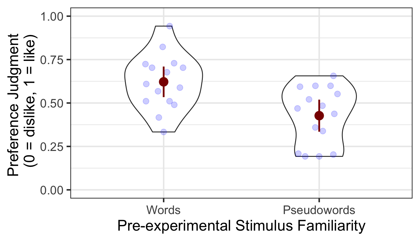
1.1.1 ANOVA
Mean preference scores were submitted to a one-way ANOVA. The difference between conditions was statistically significant. The preference score was higher in the words than pseudowords condition.
p1.aov <- aov_ez(id = "SID", dv = "Preference", data = P1slong, between = "Familiarity")
anova(p1.aov, es = "pes") %>% kable(digits = 4)| num Df | den Df | MSE | F | pes | Pr(>F) | |
|---|---|---|---|---|---|---|
| Familiarity | 1 | 28 | 0.0265 | 10.7292 | 0.277 | 0.0028 |
2 Item-Source Association Phase
Participants learned 48 item-location (a quadrant on the screen) associations. They were instructed to pay attention to the location of each item while making a preference judgment. A between-participants pre-experimental stimulus familiarity factor determined whether a participant was exposed to words or pseudowords. A within-participant item repetition factor determined whether a repeated item (which had been presented in the first phase) or an unrepeated item (which appeared for the first time in the item-source association phase) was presented in each trial.
P2 <- read.csv("data/data_FamSM_Exp2_Word_SRC.csv", header = T)
P2$Familiarity = factor(P2$Familiarity, levels=c(1,2), labels=c("Words","Pseudowords"))
P2$Repetition = factor(P2$Repetition, levels=c(1,2), labels=c("Repeated","Unrepeated"))
P2$Pref <- ifelse(P2$Resp==1,1,0)

glimpse(P2, width=70)
## Observations: 1,440
## Variables: 10
## $ SID         <int> 1, 1, 1, 1, 1, 1, 1, 1, 1, 1, 1, 1, 1, 1, 1, 1,…
## $ Familiarity <fct> Words, Words, Words, Words, Words, Words, Words…
## $ Trial       <int> 1, 2, 3, 4, 5, 6, 7, 8, 9, 10, 11, 12, 13, 14, …
## $ Repetition  <fct> Repeated, Repeated, Unrepeated, Repeated, Unrep…
## $ Loc         <int> 3, 3, 4, 3, 4, 2, 4, 2, 1, 2, 4, 1, 1, 4, 2, 2,…
## $ Resp        <int> 2, 1, 1, 1, 1, 1, 1, 2, 1, 2, 2, 2, 1, 1, 1, 2,…
## $ Corr        <int> 1, 1, 1, 1, 1, 1, 1, 1, 1, 1, 1, 1, 1, 1, 1, 1,…
## $ RT          <dbl> 738.07, 790.33, 954.48, 710.88, 1155.16, 679.36…
## $ ImgName     <fct> wordin2_1.png, wordin2_10.png, wordin1.png, wor…
## $ Pref        <dbl> 0, 1, 1, 1, 1, 1, 1, 0, 1, 0, 0, 0, 1, 1, 1, 0,…
# 1. SID: participant ID
# 2. Familiarity: pre-experimental familiarity. 1 = words, 2 = pseudowords
# 3. Trial: 1~48
# 4. Repetition: 1 = repetition, 2 = no repetition
# 5. Loc: location (source) of memory item; quadrants, 1~4
# 6. Resp: preference judgment, 1 = like, 2 = dislike, 0 = no response
# 7. Corr: correctness, 1 = response, 0 = no response
# 8. RT: reaction times in ms.
# 9. ImgName: name of stimuli
# 10. Pref: preference, 0 = dislike (treating no response as 'dislike'), 1 = like

table(P2$Familiarity, P2$SID)
##
##                1  2  3  4  5  6  7  8  9 10 11 12 13 14 15 16 17 18 19 20
##   Words       48 48 48 48 48 48 48 48 48 48 48 48 48 48 48  0  0  0  0  0
##   Pseudowords  0  0  0  0  0  0  0  0  0  0  0  0  0  0  0 48 48 48 48 48
##
##               21 22 23 24 25 26 27 28 29 30
##   Words        0  0  0  0  0  0  0  0  0  0
##   Pseudowords 48 48 48 48 48 48 48 48 48 48
table(P2$Repetition, P2$SID)
##
##               1  2  3  4  5  6  7  8  9 10 11 12 13 14 15 16 17 18 19 20
##   Repeated   24 24 24 24 24 24 24 24 24 24 24 24 24 24 24 24 24 24 24 24
##   Unrepeated 24 24 24 24 24 24 24 24 24 24 24 24 24 24 24 24 24 24 24 24
##
##              21 22 23 24 25 26 27 28 29 30
##   Repeated   24 24 24 24 24 24 24 24 24 24
##   Unrepeated 24 24 24 24 24 24 24 24 24 24

1 - mean(P2$Corr)
## [1] 0.01041667
Participants did not make responses in 1.04% of trials.
2.1 Preference
We calculated the mean and s.d. of individual participants’ preference scores for each condition. After repetition, preference decreased for words but increased for pseudowords.
P2slong <- P2 %>% group_by(SID, Familiarity, Repetition) %>%
  summarise(Preference = mean(Pref)) %>%
  ungroup()

# summary table
P2g <- P2slong %>% group_by(Familiarity, Repetition) %>%
  summarise(M = mean(Preference), SD = sd(Preference)) %>%
  ungroup()
P2g %>% kable()| Familiarity | Repetition | M | SD |
|---|---|---|---|
| Words | Repeated | 0.5972222 | 0.1664185 |
| Words | Unrepeated | 0.6722222 | 0.1934356 |
| Pseudowords | Repeated | 0.4416667 | 0.1766363 |
| Pseudowords | Unrepeated | 0.3611111 | 0.1847796 |
# group level, needed for printing & geom_pointrange
# Rmisc must be called indirectly due to incompatibility between plyr and dplyr.
P2g$ci <- Rmisc::summarySEwithin(data = P2slong, measurevar = "Preference", idvar = "SID",
                              withinvars = "Repetition", betweenvars = "Familiarity")$ci
P2g$Preference <- P2g$M

ggplot(data=P2slong, aes(x=Familiarity, y=Preference, fill=Repetition)) +
  geom_violin(width = 0.7, trim=TRUE) +
  ggbeeswarm::geom_quasirandom(dodge.width = 0.7, color = "blue", size = 3, alpha = 0.2,
                               show.legend = FALSE) +
  geom_pointrange(data=P2g,
                  aes(x = Familiarity, ymin = Preference-ci, ymax = Preference+ci, color = Repetition),
                  position = position_dodge(0.7), color = "darkred", size = 1, show.legend = FALSE) +
  coord_cartesian(ylim = c(0, 1), clip = "on") +
  labs(x = "Pre-experimental Stimulus Familiarity",
       y = "Preference Judgment \n (0 = dislike, 1 = like)",
       fill='Item Repetition') +
  scale_fill_manual(values=c("#E69F00", "#56B4E9"),
                    labels=c("Repeated", "Unrepeated")) +
  theme_bw(base_size = 18) +
  theme(panel.grid.major = element_blank(),
panel.grid.minor = element_blank()) 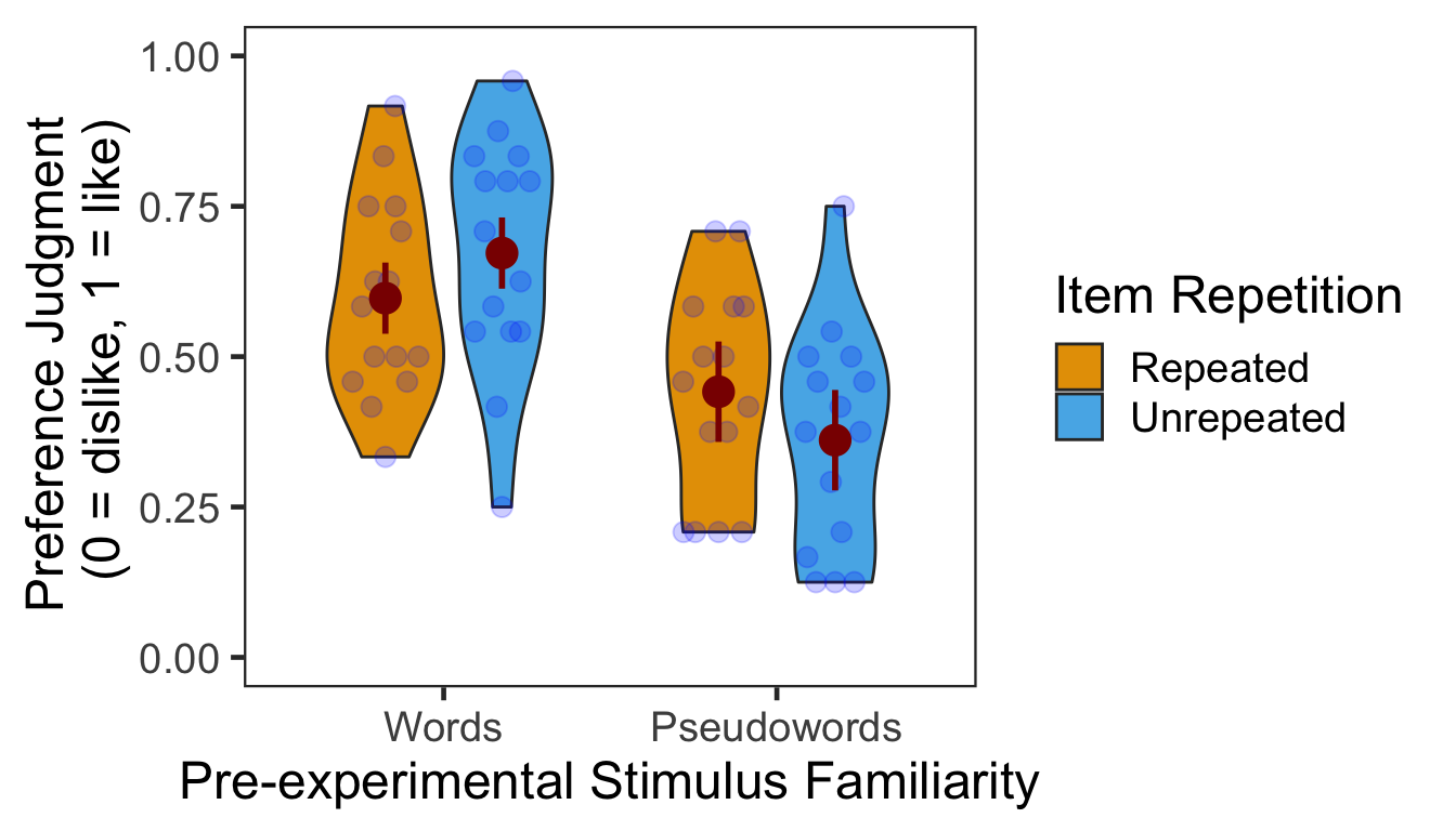
2.1.1 ANOVA
We performed a 2x2 mixed design ANOVA with pre-experimental stimulus familiarity as a between-participants factor and item repetition as a within-participant factor. The main effect of pre-experimental stimulus familiarity and the two-way interaction were both significant.
p2.aov <- aov_ez(id = "SID", dv = "Preference", data = P2slong,
                 between = "Familiarity", within = "Repetition")
anova(p2.aov, es = "pes") %>% kable(digits = 4)| num Df | den Df | MSE | F | pes | Pr(>F) | |
|---|---|---|---|---|---|---|
| Familiarity | 1 | 28 | 0.0481 | 16.9659 | 0.3773 | 0.0003 |
| Repetition | 1 | 28 | 0.0171 | 0.0068 | 0.0002 | 0.9350 |
| Familiarity:Repetition | 1 | 28 | 0.0171 | 5.3088 | 0.1594 | 0.0289 |
As post-hoc analyses, we performed two one-way repeated measures ANOVAs to contrast repeated vs. unrepeated items within each pre-experimental stimulus familiarity condition. The first table shows the results from the words condition and the second table shows the results from the pseudowords condition.
p2.pref.aov.r1 <- aov_ez(id = "SID", dv = "Preference", within = "Repetition",
                        data = filter(P2slong, Familiarity == "Words"))
anova(p2.pref.aov.r1, es = "pes") %>% kable(digits = 4)| num Df | den Df | MSE | F | pes | Pr(>F) | |
|---|---|---|---|---|---|---|
| Repetition | 1 | 14 | 0.0114 | 3.6898 | 0.2086 | 0.0753 |
Item repetition tended to reduce preference for words.
p2.pref.aov.r2 <- aov_ez(id = "SID", dv = "Preference", within = "Repetition",
                        data = filter(P2slong, Familiarity == "Pseudowords"))
anova(p2.pref.aov.r2, es = "pes") %>% kable(digits = 4)| num Df | den Df | MSE | F | pes | Pr(>F) | |
|---|---|---|---|---|---|---|
| Repetition | 1 | 14 | 0.0228 | 2.1392 | 0.1325 | 0.1657 |
Item repetition did not significantly affect preference for pseudowords.
3 Source Memory Test Phase
In each trial, participants first indicated in which quadrant a given item appeared during the item-source association phase. Participants then rated how confident they were about their memory judgment. There were 48 trials in total.
P3 <- read.csv("data/data_FamSM_Exp2_Word_TST.csv", header = T)
P3$Familiarity = factor(P3$Familiarity, levels=c(1,2), labels=c("Words","Pseudowords"))
P3$Repetition = factor(P3$Repetition, levels=c(1,2), labels=c("Repeated","Unrepeated"))

glimpse(P3, width=70)
## Observations: 1,440
## Variables: 10
## $ SID         <int> 1, 1, 1, 1, 1, 1, 1, 1, 1, 1, 1, 1, 1, 1, 1, 1,…
## $ Familiarity <fct> Words, Words, Words, Words, Words, Words, Words…
## $ Trial       <int> 1, 2, 3, 4, 5, 6, 7, 8, 9, 10, 11, 12, 13, 14, …
## $ Repetition  <fct> Repeated, Unrepeated, Repeated, Unrepeated, Rep…
## $ AscLoc      <int> 3, 4, 3, 1, 1, 2, 4, 1, 1, 2, 2, 2, 1, 2, 2, 3,…
## $ ScrResp     <int> 3, 2, 2, 1, 1, 2, 4, 1, 1, 2, 2, 1, 1, 2, 2, 3,…
## $ Corr        <int> 1, 0, 0, 1, 1, 1, 1, 1, 1, 1, 1, 0, 1, 1, 1, 1,…
## $ RT          <dbl> 2463.98, 2449.93, 2174.49, 1781.44, 1815.03, 12…
## $ Confident   <int> 4, 4, 4, 4, 4, 4, 4, 4, 4, 1, 4, 2, 2, 3, 4, 2,…
## $ ImgName     <fct> wordin2_8.png, wordex7.png, wordex8.png, wordin…
# 1. SID: participant ID
# 2. Familiarity: pre-experimental familiarity. 1 = words, 2 = pseudowords
# 3. Trial: 1~48
# 4. Repetition: 1 = repetition, 2 = no repetition
# 5. AscLoc: location (source) in which the item was presented in Phase 2; quadrants, 1~4
# 6. SrcResp: source response; quadrants, 1~4
# 7. Corr: correctness, 1=correct, 0=incorrect
# 8. RT: reaction times in ms.
# 9. Confident: confidence rating, 1~4
# 10. ImgName: name of stimuli

table(P3$Familiarity, P3$SID)
##
##                1  2  3  4  5  6  7  8  9 10 11 12 13 14 15 16 17 18 19 20
##   Words       48 48 48 48 48 48 48 48 48 48 48 48 48 48 48  0  0  0  0  0
##   Pseudowords  0  0  0  0  0  0  0  0  0  0  0  0  0  0  0 48 48 48 48 48
##
##               21 22 23 24 25 26 27 28 29 30
##   Words        0  0  0  0  0  0  0  0  0  0
##   Pseudowords 48 48 48 48 48 48 48 48 48 48
table(P3$Repetition, P3$SID)
##
##               1  2  3  4  5  6  7  8  9 10 11 12 13 14 15 16 17 18 19 20
##   Repeated   24 24 24 24 24 24 24 24 24 24 24 24 24 24 24 24 24 24 24 24
##   Unrepeated 24 24 24 24 24 24 24 24 24 24 24 24 24 24 24 24 24 24 24 24
##
##              21 22 23 24 25 26 27 28 29 30
##   Repeated   24 24 24 24 24 24 24 24 24 24
##   Unrepeated 24 24 24 24 24 24 24 24 24 24
3.1 Accuracy
We calculated the mean and s.d. of individual participants’ mean percentage accuracy. In the following plot, red points and error bars represent the means and 95% within-participants CIs.
# phase 3, subject-level, long-format
P3ACCslong <- P3 %>% group_by(SID, Familiarity, Repetition) %>%
  summarise(Accuracy = mean(Corr)*100) %>%
  ungroup()

# summary table
P3ACCg <- P3ACCslong %>% group_by(Familiarity, Repetition) %>%
  summarise(M = mean(Accuracy), SD = sd(Accuracy)) %>%
  ungroup()
P3ACCg %>% kable()| Familiarity | Repetition | M | SD |
|---|---|---|---|
| Words | Repeated | 56.11111 | 15.25792 |
| Words | Unrepeated | 75.55556 | 17.80813 |
| Pseudowords | Repeated | 52.77778 | 14.49092 |
| Pseudowords | Unrepeated | 45.83333 | 11.13589 |
# marginal means of famous vs. non-famous conditions.
P3ACCslong %>% group_by(Familiarity) %>%
  summarise(M = mean(Accuracy), SD = sd(Accuracy)) %>%
ungroup() %>% kable()| Familiarity | M | SD |
|---|---|---|
| Words | 65.83333 | 19.05955 |
| Pseudowords | 49.30556 | 13.17994 |
# marginal means of repeated vs. unrepeated conditions.
P3ACCslong %>% group_by(Repetition) %>%
  summarise(M = mean(Accuracy), SD = sd(Accuracy)) %>%
ungroup() %>% kable()| Repetition | M | SD |
|---|---|---|
| Repeated | 54.44444 | 14.71852 |
| Unrepeated | 60.69444 | 21.01026 |
# wide format, needed for geom_segments.
P3ACCswide <- P3ACCslong %>% spread(key = Repetition, value = Accuracy)

# group level, needed for printing & geom_pointrange
# Rmisc must be called indirectly due to incompatibility between plyr and dplyr.
P3ACCg$ci <- Rmisc::summarySEwithin(data = P3ACCslong, measurevar = "Accuracy", idvar = "SID",
                                    withinvars = "Repetition", betweenvars = "Familiarity")$ci
P3ACCg$Accuracy <- P3ACCg$M

ggplot(data=P3ACCslong, aes(x=Familiarity, y=Accuracy, fill=Repetition)) +
  geom_violin(width = 0.5, trim=TRUE) +
  geom_point(position=position_dodge(0.5), color="gray80", size=1.8, show.legend = FALSE) +
  geom_segment(data=filter(P3ACCswide, Familiarity=="Words"), inherit.aes = FALSE,
               aes(x=1-.12, y=filter(P3ACCswide, Familiarity=="Words")$Repeated,
                   xend=1+.12, yend=filter(P3ACCswide, Familiarity=="Words")$Unrepeated),
               color="gray80") +
  geom_segment(data=filter(P3ACCswide, Familiarity=="Pseudowords"), inherit.aes = FALSE,
               aes(x=2-.12, y=filter(P3ACCswide, Familiarity=="Pseudowords")$Repeated,
                   xend=2+.12, yend=filter(P3ACCswide, Familiarity=="Pseudowords")$Unrepeated),
               color="gray80") +
  geom_pointrange(data=P3ACCg,
                  aes(x = Familiarity, ymin = Accuracy-ci, ymax = Accuracy+ci, group = Repetition),
                  position = position_dodge(0.5), color = "darkred", size = 1, show.legend = FALSE) +
  scale_fill_manual(values=c("#E69F00", "#56B4E9"),
                    labels=c("Repeated", "Unrepeated")) +
  labs(x = "Pre-experimental Stimulus Familiarity",
       y = "Source Memory Accuracy (%)",
       fill='Item Repetition') +
  coord_cartesian(ylim = c(0, 100), clip = "on") +
  theme_bw(base_size = 18) +
  theme(panel.grid.major = element_blank(),
panel.grid.minor = element_blank()) 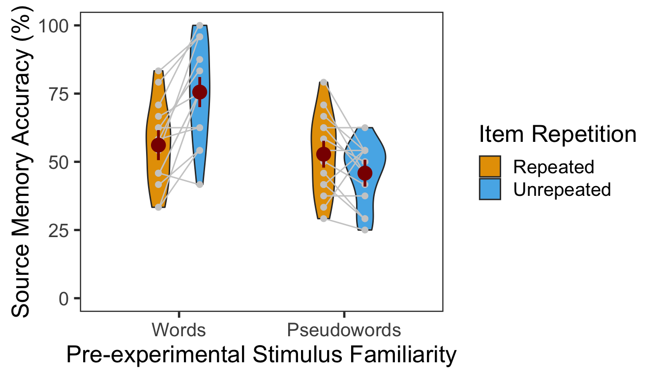
The effect of item repetition was modulated by the pre-experimental stimulus familiarity of the items. For words, the locations of unrepeated items were better remembered (novelty effect). For pseudowords, the locations of repeated items were better remembered (familiarity effect). These crossed effects were on top of the general familiarity effect, in which source memory was more accurate for words than for pseudowords.
3.1.1 ANOVA
Individuals’ mean percentage accuracy was submitted to a 2x2 mixed design ANOVA with pre-experimental stimulus familiarity as a between-participants factor (words vs. pseudowords) and item repetition as a within-participant factor (repeated vs. unrepeated).
p3.corr.aov <- aov_ez(id = "SID", dv = "Accuracy", data = P3ACCslong,
                 between = "Familiarity", within = "Repetition")
anova(p3.corr.aov, es = "pes") %>% kable(digits = 4)| num Df | den Df | MSE | F | pes | Pr(>F) | |
|---|---|---|---|---|---|---|
| Familiarity | 1 | 28 | 353.0919 | 11.6047 | 0.2930 | 0.0020 |
| Repetition | 1 | 28 | 88.8724 | 6.5930 | 0.1906 | 0.0159 |
| Familiarity:Repetition | 1 | 28 | 88.8724 | 29.3837 | 0.5121 | 0.0000 |
Both main effects were significant, and so was their interaction. Then, we performed two separate one-way repeated measures ANOVAs as post-hoc analyses. In the following two tables, the first presents the effect of item repetition for words, and the second presents the same effect for pseudowords.
ci95 <- P3ACCswide %>% filter(Familiarity=="Words") %>%
  mutate(Diff = Unrepeated - Repeated) %>%
  summarise(lower = mean(Diff) - qt(0.975,df=n()-1)*sd(Diff)/sqrt(n()),
            upper = mean(Diff) + qt(0.975,df=n()-1)*sd(Diff)/sqrt(n()))

p3.corr.aov.r1 <- aov_ez(id = "SID", dv = "Accuracy", within = "Repetition",
                        data = filter(P3ACCslong, Familiarity == "Words"))
anova(p3.corr.aov.r1, es = "pes") %>% kable(digits = 4)| num Df | den Df | MSE | F | pes | Pr(>F) | |
|---|---|---|---|---|---|---|
| Repetition | 1 | 14 | 98.793 | 28.7029 | 0.6722 | 1e-04 |
In the words group, source memory accuracy was higher for unrepeated than repeated items. The 95% CI of difference between the means was [11.66, 27.23].
ci95 <- P3ACCswide %>% filter(Familiarity=="Pseudowords") %>%
  mutate(Diff = Repeated - Unrepeated) %>%
  summarise(lower = mean(Diff) - qt(0.975,df=n()-1)*sd(Diff)/sqrt(n()),
            upper = mean(Diff) + qt(0.975,df=n()-1)*sd(Diff)/sqrt(n()))

p3.corr.aov.r2 <- aov_ez(id = "SID", dv = "Accuracy", within = "Repetition",
                        data = filter(P3ACCslong, Familiarity == "Pseudowords"))
anova(p3.corr.aov.r2, es = "pes") %>% kable(digits = 4)| num Df | den Df | MSE | F | pes | Pr(>F) | |
|---|---|---|---|---|---|---|
| Repetition | 1 | 14 | 78.9517 | 4.5812 | 0.2465 | 0.0504 |
In the pseudowords group, source memory tended to be more accurate for repeated than unrepeated items. The 95% CI of difference between the means was [-0.01, 13.9].
3.1.2 GLMM
To supplement conventional ANOVAs, we tested generalized linear mixed models (GLMM) on source memory accuracy. This mixed modeling approach with a binomial link function is expected to properly handle binary data such as source memory responses (i.e., correct or not; Jaeger, 2008).
We built the full model (full1) with two fixed effects (pre-experimental stimulus familiarity and item repetition) and their interaction. The model also included maximal random effects structure (Barr, Levy, Scheepers, & Tily, 2013): both by-participant and by-item random intercepts, and by-participant random slopes for item repetition. In case the maximal model does not converge successfully, we built another model (full2) with the maximal random structure but with the correlations among the random terms removed (Singmann, 2018).
To fit the models, we used the mixed() of the afex package (Singmann, Bolker, & Westfall, 2017) which was built on the lmer() of the lme4 package (Bates, Maechler, Bolker, & Walker, 2015). The mixed() assessed the statistical significance of fixed effects by comparing a model with the effect in question against its nested model which lacked the effect in question. P-values of the effects were obtained by likelihood ratio tests (LRT).
(nc <- detectCores())
cl <- makeCluster(rep("localhost", nc))

full1 <- afex::mixed(Corr ~ Familiarity*Repetition + (Repetition|SID) + (1|ImgName),
               P3, method = "LRT", cl = cl,
               family=binomial(link="logit"),
               control = glmerControl(optCtrl = list(maxfun = 1e6)))
full2 <- afex::mixed(Corr ~ Familiarity*Repetition + (Repetition||SID) + (1|ImgName),
               P3, method = "LRT", cl = cl,
               family=binomial(link="logit"),
               control = glmerControl(optCtrl = list(maxfun = 1e6)), expand_re = TRUE)

stopCluster(cl)
The table below presents the LRT results of the models full1 and full2.
full.compare <- cbind(afex::nice(full1), afex::nice(full2)[,-c(1,2)])
colnames(full.compare)[c(3,4,5,6)] <- c("full1 Chisq", "p","full2 Chisq", "p")
full.compare %>% kable()| Effect | df | full1 Chisq | p | full2 Chisq | p |
|---|---|---|---|---|---|
| Familiarity | 1 | 10.45 ** | .001 | 10.38 ** | .001 |
| Repetition | 1 | 8.27 ** | .004 | 7.78 ** | .005 |
| Familiarity:Repetition | 1 | 22.42 *** | <.0001 | 22.07 *** | <.0001 |
The p-values from the two models were highly similar to each other. Post-hoc analysis results are summarized in the table below. The results from the pairwise comparisons were consistent with those from the ANOVA. Item repetition significantly impaired source memory for words whereas it slightly improved source memory for pseudowords.
emmeans(full1, pairwise ~ Repetition | Familiarity, type = "response")$contrasts %>% kable()| contrast | Familiarity | odds.ratio | SE | df | z.ratio | p.value |
|---|---|---|---|---|---|---|
| Repeated / Unrepeated | Words | 0.3695639 | 0.0669653 | Inf | -5.493526 | 0.0000000 |
| Repeated / Unrepeated | Pseudowords | 1.3417218 | 0.2136544 | Inf | 1.845991 | 0.0648935 |
3.2 Confidence
The table below shows the mean and s.d. of individual participants’ confidence ratings for each condition. The pattern of confidence ratings was qualitatively identical to that of source memory accuracy; we observed the novelty benefit for words and the familiarity benefit for pseudowords.
P3CFslong <- P3 %>% group_by(SID, Familiarity, Repetition) %>%
  summarise(Confidence = mean(Confident)) %>%
  ungroup()

P3CFg <- P3CFslong %>%
  group_by(Familiarity, Repetition) %>%
  summarise(M = mean(Confidence), SD = sd(Confidence)) %>%
  ungroup()
P3CFg %>% kable()| Familiarity | Repetition | M | SD |
|---|---|---|---|
| Words | Repeated | 2.472222 | 0.3846853 |
| Words | Unrepeated | 3.180556 | 0.4926712 |
| Pseudowords | Repeated | 2.611111 | 0.4860828 |
| Pseudowords | Unrepeated | 2.269444 | 0.4187053 |
# marginal means of famous vs. non-famous conditions.
P3CFslong %>% group_by(Familiarity) %>%
  summarise(M = mean(Confidence), SD = sd(Confidence)) %>%
ungroup() %>% kable()| Familiarity | M | SD |
|---|---|---|
| Words | 2.826389 | 0.5642489 |
| Pseudowords | 2.440278 | 0.4784238 |
# marginal means of repeated vs. unrepeated conditions.
P3CFslong %>% group_by(Repetition) %>%
  summarise(M = mean(Confidence), SD = sd(Confidence)) %>%
ungroup() %>% kable()| Repetition | M | SD |
|---|---|---|
| Repeated | 2.541667 | 0.4364554 |
| Unrepeated | 2.725000 | 0.6453674 |
# wide format, needed for geom_segments.
P3CFswide <- P3CFslong %>% spread(key = Repetition, value = Confidence)

# group level, needed for printing & geom_pointrange
# Rmisc must be called indirectly due to incompatibility between plyr and dplyr.
P3CFg$ci <- Rmisc::summarySEwithin(data = P3CFslong, measurevar = "Confidence", idvar = "SID",
                                   withinvars = "Repetition", betweenvars = "Familiarity")$ci
P3CFg$Confidence <- P3CFg$M

ggplot(data=P3CFslong, aes(x=Familiarity, y=Confidence, fill=Repetition)) +
  geom_violin(width = 0.5, trim=TRUE) +
  geom_point(position=position_dodge(0.5), color="gray80", size=1.8, show.legend = FALSE) +
  geom_segment(data=filter(P3CFswide, Familiarity=="Words"), inherit.aes = FALSE,
               aes(x=1-.12, y=filter(P3CFswide, Familiarity=="Words")$Repeated,
                   xend=1+.12, yend=filter(P3CFswide, Familiarity=="Words")$Unrepeated),
               color="gray80") +
  geom_segment(data=filter(P3CFswide, Familiarity=="Pseudowords"), inherit.aes = FALSE,
               aes(x=2-.12, y=filter(P3CFswide, Familiarity=="Pseudowords")$Repeated,
                   xend=2+.12, yend=filter(P3CFswide, Familiarity=="Pseudowords")$Unrepeated),
               color="gray80") +
  geom_pointrange(data=P3CFg,
                  aes(x = Familiarity, ymin = Confidence-ci, ymax = Confidence+ci, group = Repetition),
                  position = position_dodge(0.5), color = "darkred", size = 1, show.legend = FALSE) +
  scale_fill_manual(values=c("#E69F00", "#56B4E9"),
                    labels=c("Repeated", "Unrepeated")) +
  labs(x = "Pre-experimental Stimulus Familiarity",
       y = "Source Memory Confidence",
       fill='Item Repetition') +
  coord_cartesian(ylim = c(1, 4), clip = "on") +
  theme_bw(base_size = 18) +
  theme(panel.grid.major = element_blank(),
        panel.grid.minor = element_blank())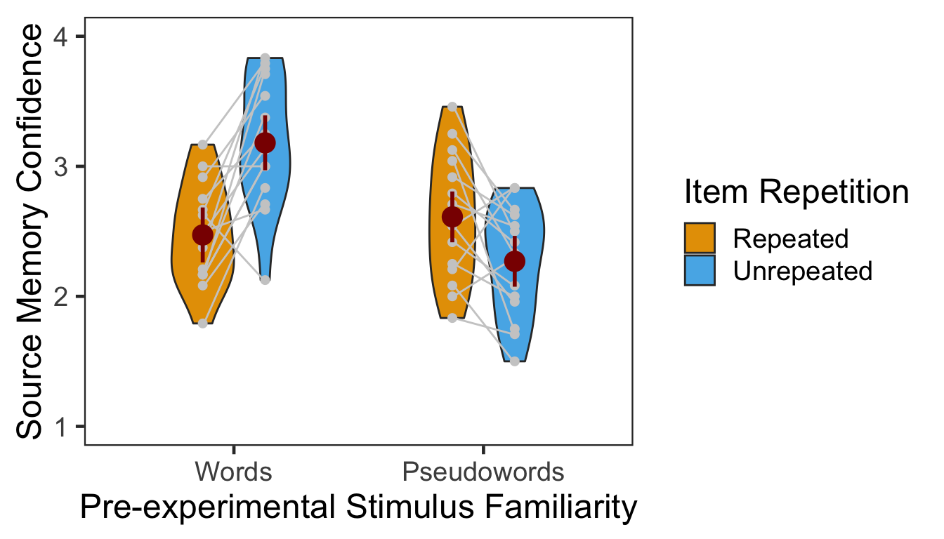
3.2.1 ANOVA
Individuals’ confidence ratings were submitted to a 2x2 mixed design ANOVA with pre-experimental stimulus familiarity as a between-participants factor and item repetition as a within-participant factor.
p3.conf.aov <- aov_ez(id = "SID", dv = "Confidence", data = P3CFslong,
                      between = "Familiarity", within = "Repetition")
anova(p3.conf.aov, es = "pes") %>% kable(digits = 4)| num Df | den Df | MSE | F | pes | Pr(>F) | |
|---|---|---|---|---|---|---|
| Familiarity | 1 | 28 | 0.2661 | 8.4040 | 0.2309 | 0.0072 |
| Repetition | 1 | 28 | 0.1351 | 3.7330 | 0.1176 | 0.0635 |
| Familiarity:Repetition | 1 | 28 | 0.1351 | 30.6121 | 0.5223 | 0.0000 |
The main effect of pre-experimental stimulus familiarity and the two-way interaction were both significant. The main effect of item repetition was marginally significant. Next we performed two additional one-way repeated measures ANOVAs as post-hoc analyses. The first table below presents the effect of item repetition for words, and the second presents the same effect for pseudowords. The results showed that item repetition had significant effects on confidence ratings for words vs. pseudowords in opposite directions.
ci95 <- P3CFswide %>% filter(Familiarity=="Words") %>%
  mutate(Diff = Unrepeated - Repeated) %>%
  summarise(lower = mean(Diff) - qt(0.975,df=n()-1)*sd(Diff)/sqrt(n()),
            upper = mean(Diff) + qt(0.975,df=n()-1)*sd(Diff)/sqrt(n()))

p3.conf.aov.r1 <- aov_ez(id = "SID", dv = "Confidence", within = "Repetition",
                         data = filter(P3CFslong, Familiarity == "Words"))
anova(p3.conf.aov.r1, es = "pes") %>% kable(digits = 4)| num Df | den Df | MSE | F | pes | Pr(>F) | |
|---|---|---|---|---|---|---|
| Repetition | 1 | 14 | 0.1456 | 25.8475 | 0.6487 | 2e-04 |
In the word group, participants were more confident on their source memory for unrepeated than repeated items. The 95% CI of difference between the means was [0.41, 1.01].
ci95 <- P3CFswide %>% filter(Familiarity=="Pseudowords") %>%
  mutate(Diff = Repeated - Unrepeated) %>%
  summarise(lower = mean(Diff) - qt(0.975,df=n()-1)*sd(Diff)/sqrt(n()),
            upper = mean(Diff) + qt(0.975,df=n()-1)*sd(Diff)/sqrt(n()))

p3.conf.aov.r2 <- aov_ez(id = "SID", dv = "Confidence", within = "Repetition",
                         data = filter(P3CFslong, Familiarity == "Pseudowords"))
anova(p3.conf.aov.r2, es = "pes") %>% kable(digits = 4)| num Df | den Df | MSE | F | pes | Pr(>F) | |
|---|---|---|---|---|---|---|
| Repetition | 1 | 14 | 0.1245 | 7.0307 | 0.3343 | 0.019 |
In the pseudoword group, participants’ confidence ratings were higher for repeated than unrepeated items. The 95% CI of difference between the means was [0.07, 0.62].
3.2.2 CLMM
The responses from a Likert-type scale are ordinal. Especially for the rating items with numerical response formats containing four or fewer categories, it is recommended to use categorical data analysis approaches, rather than treating the responses as continuous data (Harpe, 2015).
Here we employed the cumulative link mixed modeling using the clmm() of the package ordinal (Christensen, submitted). The specification of the full model was the same as the mixed() above. To determine the statistical significance, the LRT compared models with or without the fixed effect of interest.
P3R <- P3
P3R$Confident = factor(P3R$Confident, ordered = TRUE)
P3R$SID = factor(P3R$SID)

cm.full <- clmm(Confident ~ Familiarity * Repetition + (Repetition|SID) + (1|ImgName), data=P3R)
cm.red1 <- clmm(Confident ~ Familiarity + Repetition + (Repetition|SID) + (1|ImgName), data=P3R)
cm.red2 <- clmm(Confident ~ Repetition + (Repetition|SID) + (1|ImgName), data=P3R)
cm.red3 <- clmm(Confident ~ 1 + (Repetition|SID) + (1|ImgName), data=P3R)
cm.comp <- anova(cm.full, cm.red1, cm.red2, cm.red3)
data.frame(Effect = c("Familiarity", "Repetition", "Familiarity:Repetition"),
df = 1, Chisq = cm.comp$LR.stat[2:4], p = cm.comp$`Pr(>Chisq)`[2:4]) %>% kable()| Effect | df | Chisq | p |
|---|---|---|---|
| Familiarity | 1 | 2.254686 | 0.1332104 |
| Repetition | 1 | 1.798513 | 0.1798924 |
| Familiarity:Repetition | 1 | 22.432508 | 0.0000022 |
The LRT revealed a significant two-way interaction. Neither main effects were significant. Next we performed pairwise comparisons as post-hoc analyses. As shown in the following table, the results of the pairwise comparisons were consistent with those from the ANOVA approach.
emmeans(cm.full, pairwise ~ Repetition | Familiarity)$contrasts %>% kable()| contrast | Familiarity | estimate | SE | df | z.ratio | p.value |
|---|---|---|---|---|---|---|
| Repeated - Unrepeated | Words | -1.4215576 | 0.2577894 | Inf | -5.514416 | 0.0000000 |
| Repeated - Unrepeated | Pseudowords | 0.6353083 | 0.2522257 | Inf | 2.518808 | 0.0117753 |
Below is the plot of estimated marginal means, which were extracted from the fitted CLMM. The estimated distribution of confidence ratings shows the interaction between item repetition and pre-experimental stimulus familiarity.
temp <- emmeans(cm.full,~Familiarity:Repetition|cut, mode="linear.predictor")
temp <- rating.emmeans(temp)
temp <- temp %>% unite(Condition, c("Familiarity", "Repetition"))

ggplot(data = temp, aes(x = Rating, y = Prob, group = Condition)) +
  geom_line(aes(color = Condition), size = 1.2) +
  geom_point(aes(shape = Condition, color = Condition), size = 4, fill = "white", stroke = 1.2) +
  scale_color_manual(values=c("#56B4E9", "#56B4E9", "#E69F00", "#E69F00")) +
  scale_shape_manual(name="Condition", values=c(21,24,21,24)) +
  labs(y = "Response Probability", x = "Rating") +
  expand_limits(y=0) +
  scale_y_continuous(limits = c(0, 0.6)) +
  scale_x_discrete(labels = c("1" = "1(Guessed)","4"="4(Sure)")) +
  theme_minimal() +
  theme(text = element_text(size=18))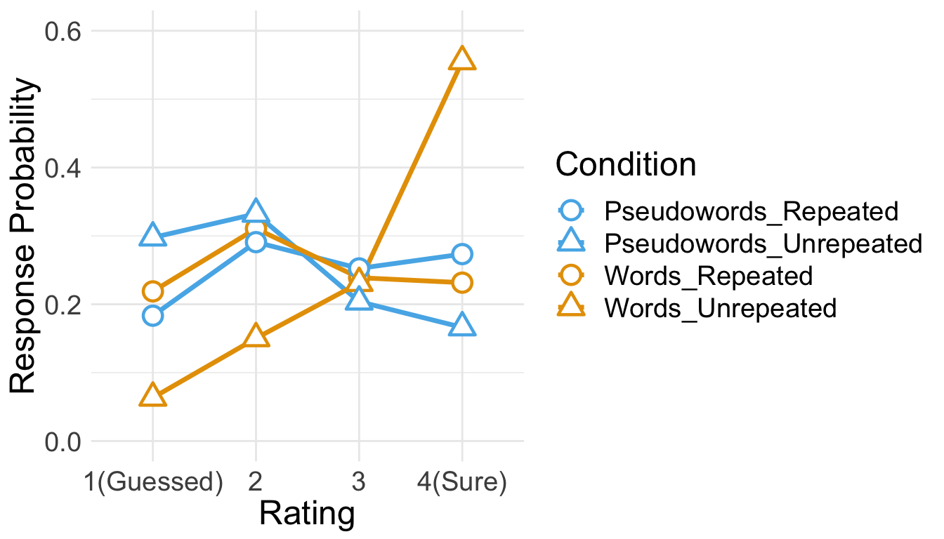
3.3 RT
Only RTs in correct trials were analyzed. Before analysis, we first removed RTs either shorter than 200ms or longer than 10s. Then, from the RT distribution of each condition, RTs beyond 3 s.d. from the mean were additionally removed.
cP3 <- P3 %>% filter(Corr==1)

sP3 <- cP3 %>% filter(RT > 200 & RT < 10000) %>%
  group_by(SID) %>%
  nest() %>%
  mutate(lbound = map(data, ~mean(.$RT)-3*sd(.$RT)),
         ubound = map(data, ~mean(.$RT)+3*sd(.$RT))) %>%
  unnest(lbound, ubound) %>%
  unnest(data) %>%
  ungroup() %>%
  mutate(Outlier = (RT < lbound)|(RT > ubound)) %>%
  filter(Outlier == FALSE) %>%
  select(SID, Familiarity, Repetition, RT, ImgName)

100 - 100*nrow(sP3)/nrow(cP3)
## [1] 3.256936
This trimming procedure removed 3.26% of correct RTs.
Since the overall source memory accuracy was not high, only small numbers of correct trials were available after trimming. The following table summarizes the numbers of trials submitted to subsequent analyses. No participant had more than 25 trials per condition.
sP3 %>% group_by(SID, Familiarity, Repetition) %>%
  summarise(NumTrial = length(RT)) %>%
  ungroup %>%
  group_by(Familiarity, Repetition) %>%
  summarise(Avg = mean(NumTrial),
            Med = median(NumTrial),
            Min = min(NumTrial),
            Max = max(NumTrial)) %>%
  ungroup %>%
kable()| Familiarity | Repetition | Avg | Med | Min | Max |
|---|---|---|---|---|---|
| Words | Repeated | 12.93333 | 14 | 7 | 18 |
| Words | Unrepeated | 17.73333 | 18 | 10 | 24 |
| Pseudowords | Repeated | 12.33333 | 12 | 7 | 19 |
| Pseudowords | Unrepeated | 10.46667 | 11 | 5 | 14 |
den1 <- ggplot(cP3, aes(x=RT)) +
  geom_density() +
  theme_bw(base_size = 18) +
  theme(panel.grid.major = element_blank(),
        panel.grid.minor = element_blank(),
        axis.text.y = element_blank(),
        axis.ticks.y = element_blank())
den2 <- ggplot(sP3, aes(x=RT)) +
  geom_density() +
  theme_bw(base_size = 18) +
  labs(x = "Trimmed RT") +
  theme(panel.grid.major = element_blank(),
        panel.grid.minor = element_blank(),
        axis.text.y = element_blank(),
        axis.ticks.y = element_blank())
den1 + den2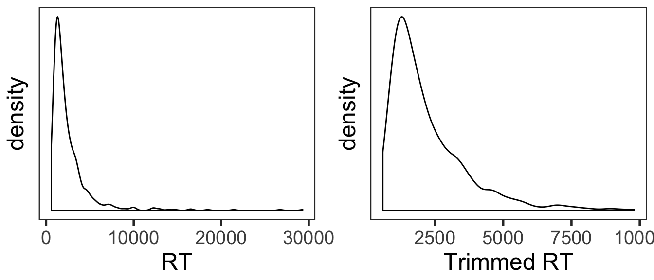
The overall RT distribution was highly skewed even after trimming. Given limited numbers of RTs and its skewed distribution, any results from the current RT analyses should be interpreted with caution and preferably corroborated with other measures.
We calculated the mean and s.d. of individual participants’ mean RTs. The overall pattern of RTs across the conditions was consistent with that of source memory accuracy and confidence ratings. In the following plot, red points and error bars represent the means and 95% within-participants CIs.
P3RTslong <- sP3 %>% group_by(SID, Familiarity, Repetition) %>%
  summarise(RT = mean(RT)) %>%
  ungroup()

P3RTg <- P3RTslong %>% group_by(Familiarity, Repetition) %>%
  summarise(M = mean(RT), SD = sd(RT)) %>%
  ungroup()
P3RTg %>% kable()| Familiarity | Repetition | M | SD |
|---|---|---|---|
| Words | Repeated | 2340.680 | 811.7648 |
| Words | Unrepeated | 1791.116 | 467.7326 |
| Pseudowords | Repeated | 2496.330 | 810.0670 |
| Pseudowords | Unrepeated | 2660.806 | 867.2041 |
# wide format, needed for geom_segments.
P3RTswide <- P3RTslong %>% spread(key = Repetition, value = RT)

# group level, needed for printing & geom_pointrange
# Rmisc must be called indirectly due to incompatibility between plyr and dplyr.
P3RTg$ci <- Rmisc::summarySEwithin(data = P3RTslong, measurevar = "RT", idvar = "SID",
                                   withinvars = "Repetition", betweenvars = "Familiarity")$ci
P3RTg$RT <- P3RTg$M

ggplot(data=P3RTslong, aes(x=Familiarity, y=RT, fill=Repetition)) +
  geom_violin(width = 0.5, trim=TRUE) +
  geom_point(position=position_dodge(0.5), color="gray80", size=1.8, show.legend = FALSE) +
  geom_segment(data=filter(P3RTswide, Familiarity=="Words"), inherit.aes = FALSE,
               aes(x=1-.12, y=filter(P3RTswide, Familiarity=="Words")$Repeated,
                   xend=1+.12, yend=filter(P3RTswide, Familiarity=="Words")$Unrepeated),
               color="gray80") +
  geom_segment(data=filter(P3RTswide, Familiarity=="Pseudowords"), inherit.aes = FALSE,
               aes(x=2-.12, y=filter(P3RTswide, Familiarity=="Pseudowords")$Repeated,
                   xend=2+.12, yend=filter(P3RTswide, Familiarity=="Pseudowords")$Unrepeated),
               color="gray80") +
  geom_pointrange(data=P3RTg,
                  aes(x = Familiarity, ymin = RT-ci, ymax = RT+ci, group = Repetition),
                  position = position_dodge(0.5), color = "darkred", size = 1, show.legend = FALSE) +
  scale_fill_manual(values=c("#E69F00", "#56B4E9"),
                    labels=c("Repeated", "Unrepeated")) +
  labs(x = "Pre-experimental Stimulus Familiarity",
       y = "Response Times (ms)",
       fill='Item Repetition') +
  theme_bw(base_size = 18) +
  theme(panel.grid.major = element_blank(),
        panel.grid.minor = element_blank())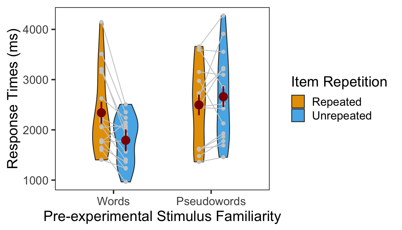
3.3.1 ANOVA
Individual participants’ mean RTs were submitted to a 2x2 mixed design ANOVA with pre-experimental stimulus familiarity as a between-participants factor and item repetition as a within-participant factor.2
p3.rt.aov <- aov_ez(id = "SID", dv = "RT", data = sP3,
                      between = "Familiarity", within = "Repetition")
anova(p3.rt.aov, es = "pes") %>% kable(digits = 4)| num Df | den Df | MSE | F | pes | Pr(>F) | |
|---|---|---|---|---|---|---|
| Familiarity | 1 | 28 | 997197.8 | 3.9535 | 0.1237 | 0.0566 |
| Repetition | 1 | 28 | 145795.8 | 3.8142 | 0.1199 | 0.0609 |
| Familiarity:Repetition | 1 | 28 | 145795.8 | 13.1139 | 0.3190 | 0.0011 |
The effect of pre-experimental stimulus familiarity was significant. Participants made faster responses to words than pseudowords. The two-way interaction was also significant. We then performed two one-way repeated-measures ANOVAs as post-hoc analyses. The first table below presents the effect of item repetition for words, and the second table presents the same effect for pseudowords.
p3.rt.aov.r1 <- aov_ez(id = "SID", dv = "RT", within = "Repetition",
                         data = filter(sP3, Familiarity == "Words"))
anova(p3.rt.aov.r1, es = "pes") %>% kable(digits = 4)| num Df | den Df | MSE | F | pes | Pr(>F) | |
|---|---|---|---|---|---|---|
| Repetition | 1 | 14 | 154366.8 | 14.6738 | 0.5118 | 0.0018 |
For words, RTs were significantly faster for unrepeated items.
p3.rt.aov.r2 <- aov_ez(id = "SID", dv = "RT", within = "Repetition",
                         data = filter(sP3, Familiarity == "Pseudowords"))
anova(p3.rt.aov.r2, es = "pes") %>% kable(digits = 4)| num Df | den Df | MSE | F | pes | Pr(>F) | |
|---|---|---|---|---|---|---|
| Repetition | 1 | 14 | 137224.9 | 1.4785 | 0.0955 | 0.2441 |
For pseudowords, RTs were marginally faster for repeated items.
3.4 Preference matters?
The pattern of preference scores in Phase 2 resembled that of the source memory accuracy and confidence ratings in Phase 3. Does this indicate that source memory performance was affected by the preference judgment? Here, we reanalyzed the data from the source memory test phase using the preference response during the item-source association phase as an additional factor.
P3$Preference <- NA
for (it in 1:nrow(P3)){
  P3$Preference[it] <- P2$Pref[ P2$SID==P3$SID[it] & P2$ImgName==P3$ImgName[it] ]
}
P3$Preference = factor(P3$Preference, levels=c(0,1), labels=c("Dislike","Like"))
3.4.1 Source Memory Accuracy
Individuals’ mean percentage accuracy was submitted to a 2x2x2 mixed design ANOVA with pre-experimental stimulus familiarity (words vs. pseudowords) as a between-participants factor and item repetition (repeated vs. unrepeated) and preference (like vs. dislike) as two within-participant factors. The main effect of preference and its interactions with the other factors were not significant.
acc.3way.aov <- aov_ez(id = "SID", dv = "Corr", data = P3,
                 between = "Familiarity", within = c("Repetition","Preference"))
anova(acc.3way.aov, es = "pes") %>% kable(digits = 4)| num Df | den Df | MSE | F | pes | Pr(>F) | |
|---|---|---|---|---|---|---|
| Familiarity | 1 | 28 | 0.0722 | 9.3724 | 0.2508 | 0.0048 |
| Repetition | 1 | 28 | 0.0243 | 5.4185 | 0.1621 | 0.0274 |
| Familiarity:Repetition | 1 | 28 | 0.0243 | 17.0639 | 0.3787 | 0.0003 |
| Preference | 1 | 28 | 0.0175 | 0.0884 | 0.0031 | 0.7684 |
| Familiarity:Preference | 1 | 28 | 0.0175 | 0.0677 | 0.0024 | 0.7966 |
| Repetition:Preference | 1 | 28 | 0.0302 | 1.6884 | 0.0569 | 0.2044 |
| Familiarity:Repetition:Preference | 1 | 28 | 0.0302 | 0.0825 | 0.0029 | 0.7760 |
apa_beeplot(data = P3,
            id="SID", dv="Corr", factors=c("Familiarity", "Repetition", "Preference"),
            dispersion = conf_int,
            ylim = c(0, 1),
            xlab = "Pre-experimental Stimulus Familiarity",
            ylab = "Source Memory Accuracy",
            args_legend = list(title = 'Item Repetition'),
            las=1)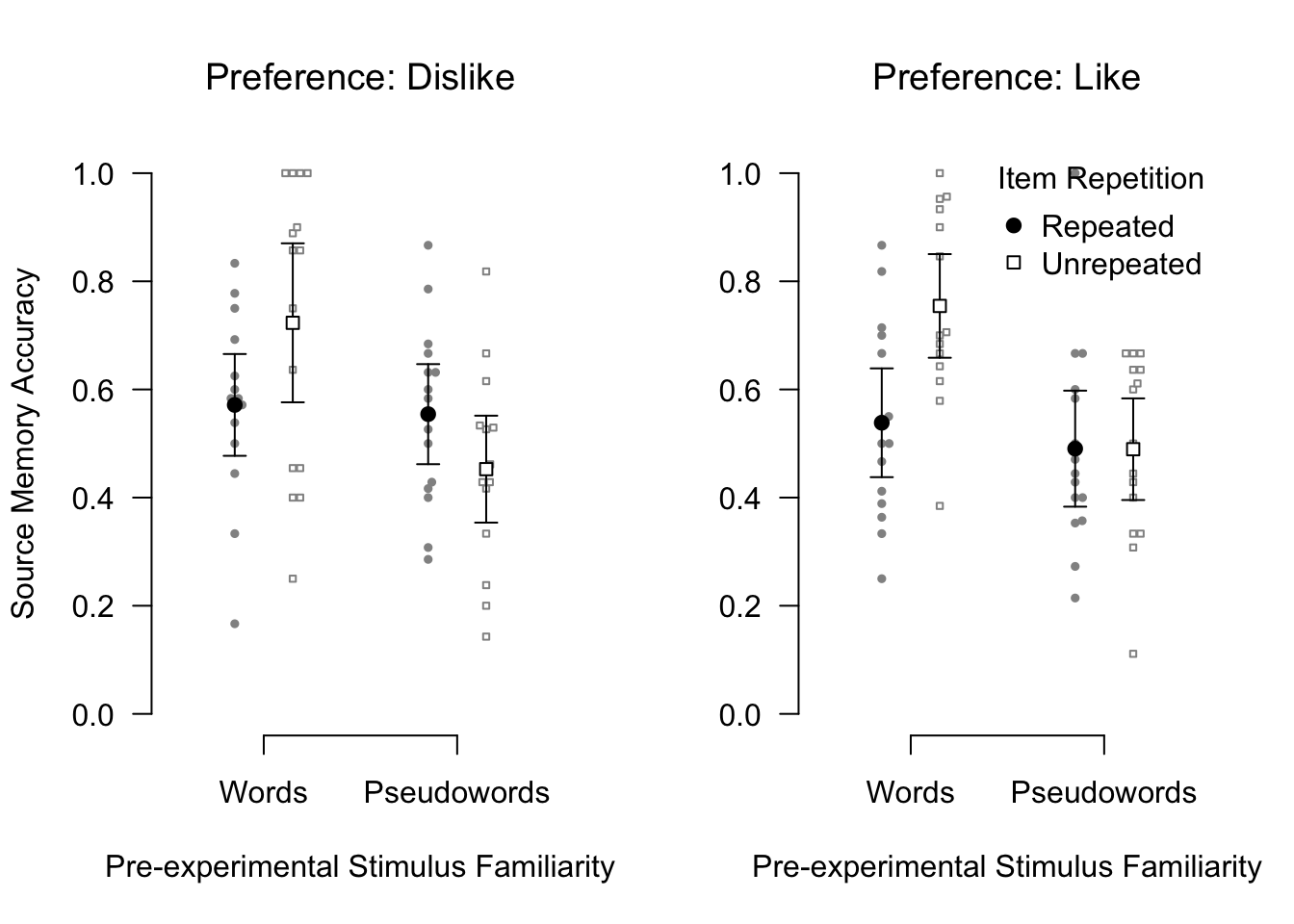
3.4.2 Source Memory Confidence
Individuals’ confidence ratings were submitted to a 2x2x2 mixed design ANOVA with pre-experimental stimulus familiarity (words vs. pseudowords) as a between-participants factor and item repetition (repeated vs. unrepeated) and preference (like vs. dislike) as two within-participant factors. The main effect of preference was significant. More importantly, however, preference did not significantly interact with any of the other factors.
conf.3way.aov <- aov_ez(id = "SID", dv = "Confident", data = P3,
                      between = "Familiarity", within = c("Repetition","Preference"))
anova(conf.3way.aov, es = "pes") %>% kable(digits = 4)| num Df | den Df | MSE | F | pes | Pr(>F) | |
|---|---|---|---|---|---|---|
| Familiarity | 1 | 28 | 0.6539 | 4.2530 | 0.1319 | 0.0486 |
| Repetition | 1 | 28 | 0.2673 | 3.7623 | 0.1185 | 0.0626 |
| Familiarity:Repetition | 1 | 28 | 0.2673 | 25.0946 | 0.4726 | 0.0000 |
| Preference | 1 | 28 | 0.1589 | 6.1510 | 0.1801 | 0.0194 |
| Familiarity:Preference | 1 | 28 | 0.1589 | 0.9715 | 0.0335 | 0.3328 |
| Repetition:Preference | 1 | 28 | 0.0973 | 1.5304 | 0.0518 | 0.2263 |
| Familiarity:Repetition:Preference | 1 | 28 | 0.0973 | 0.6308 | 0.0220 | 0.4337 |
apa_beeplot(data = P3,
            id="SID", dv="Confident", factors=c("Familiarity", "Repetition", "Preference"),
            dispersion = conf_int,
            ylim = c(0, 4),
            xlab = "Pre-experimental Stimulus Familiarity",
            ylab = "Source Memory Confidence",
            args_legend = list(title = 'Item Repetition',
                               x = "bottom", inset = 0.05),
            las=1)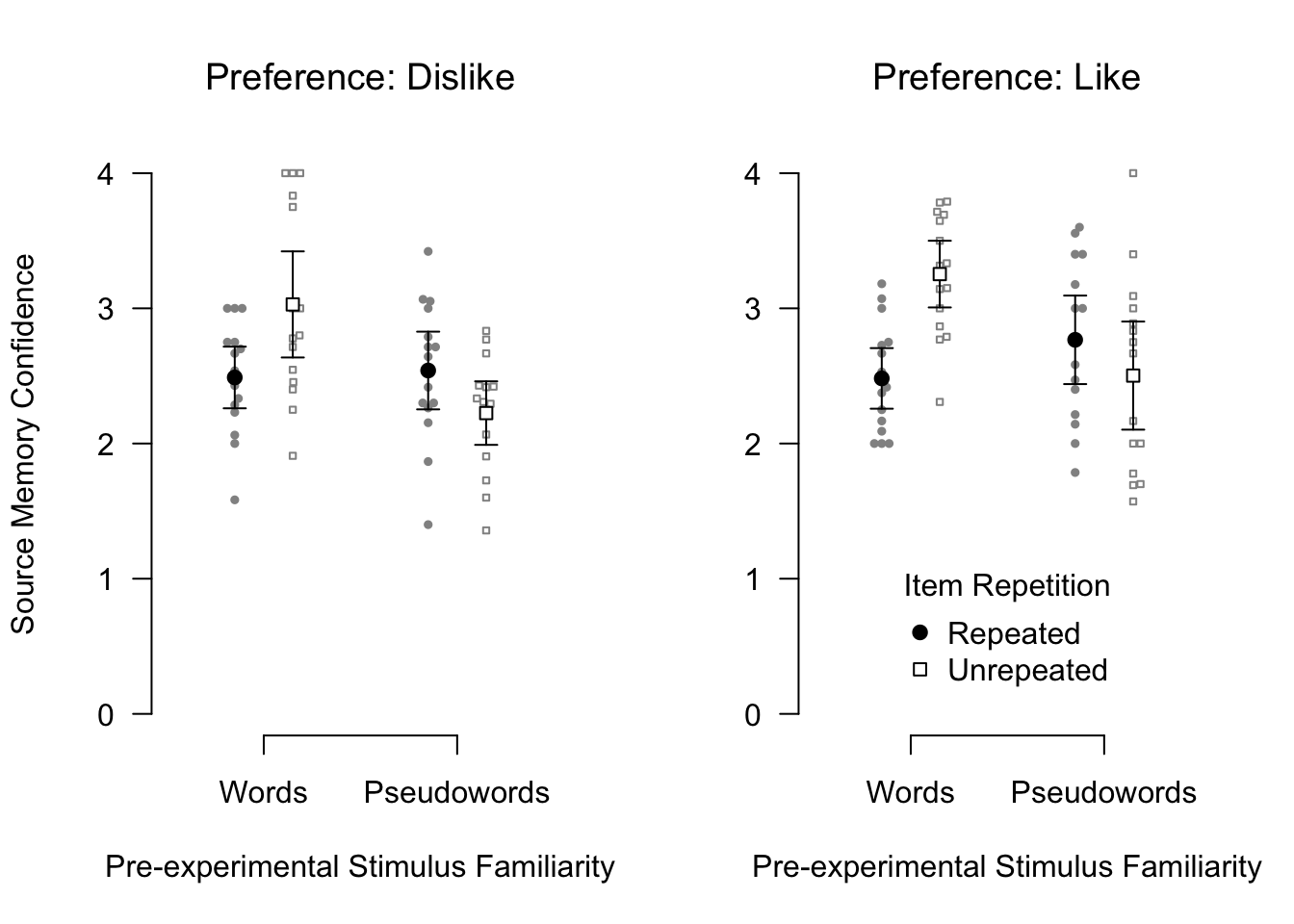
For both accuracy and confidence of source memory, no interaction with preference reached statistical significance. In contrast, the interaction between pre-experimental stimulus familiarity and item repetition remained significant. These results strongly suggest that preference alone cannot account for the interaction between pre-experimental stimulus familiarity and item repetition on source memory performance.
4 Session Info
sessionInfo()
## R version 3.5.2 (2018-12-20)
## Platform: x86_64-apple-darwin15.6.0 (64-bit)
## Running under: macOS High Sierra 10.13.6
##
## Matrix products: default
## BLAS: /Library/Frameworks/R.framework/Versions/3.5/Resources/lib/libRblas.0.dylib
## LAPACK: /Library/Frameworks/R.framework/Versions/3.5/Resources/lib/libRlapack.dylib
##
## locale:
## [1] en_US.UTF-8/en_US.UTF-8/en_US.UTF-8/C/en_US.UTF-8/en_US.UTF-8
##
## attached base packages:
## [1] parallel  stats     graphics  grDevices utils     datasets  methods
## [8] base
##
## other attached packages:
##  [1] klippy_0.0.0.9500    patchwork_0.0.1      papaja_0.1.0.9842
##  [4] RVAideMemoire_0.9-73 ggbeeswarm_0.6.0     ordinal_2019.3-9
##  [7] emmeans_1.3.3        afex_0.23-0          lme4_1.1-21
## [10] Matrix_1.2-17        car_3.0-2            carData_3.0-2
## [13] knitr_1.22           forcats_0.4.0        stringr_1.4.0
## [16] dplyr_0.8.0.1        purrr_0.3.2          readr_1.3.1
## [19] tidyr_0.8.3          tibble_2.1.1         ggplot2_3.1.0
## [22] tidyverse_1.2.1      Rmisc_1.5            plyr_1.8.4
## [25] lattice_0.20-38      pacman_0.5.1
##
## loaded via a namespace (and not attached):
##  [1] nlme_3.1-137      lubridate_1.7.4   httr_1.4.0
##  [4] numDeriv_2016.8-1 tools_3.5.2       backports_1.1.3
##  [7] utf8_1.1.4        R6_2.4.0          vipor_0.4.5
## [10] lazyeval_0.2.2    colorspace_1.4-1  withr_2.1.2
## [13] tidyselect_0.2.5  curl_3.3          compiler_3.5.2
## [16] cli_1.1.0         rvest_0.3.2       xml2_1.2.0
## [19] sandwich_2.5-0    labeling_0.3      scales_1.0.0
## [22] mvtnorm_1.0-10    digest_0.6.18     foreign_0.8-71
## [25] minqa_1.2.4       rmarkdown_1.12    rio_0.5.16
## [28] pkgconfig_2.0.2   htmltools_0.3.6   highr_0.8
## [31] rlang_0.3.3       readxl_1.3.1      rstudioapi_0.10
## [34] generics_0.0.2    zoo_1.8-5         jsonlite_1.6
## [37] zip_2.0.1         magrittr_1.5      fansi_0.4.0
## [40] Rcpp_1.0.1        munsell_0.5.0     abind_1.4-5
## [43] ucminf_1.1-4      stringi_1.4.3     multcomp_1.4-10
## [46] yaml_2.2.0        MASS_7.3-51.3     grid_3.5.2
## [49] crayon_1.3.4      haven_2.1.0       splines_3.5.2
## [52] hms_0.4.2         pillar_1.3.1      boot_1.3-20
## [55] estimability_1.3  reshape2_1.4.3    codetools_0.2-16
## [58] glue_1.3.1        evaluate_0.13     data.table_1.12.0
## [61] modelr_0.1.4      nloptr_1.2.1      cellranger_1.1.0
## [64] gtable_0.3.0      assertthat_0.2.1  xfun_0.6
## [67] openxlsx_4.1.0    xtable_1.8-3      broom_0.5.1
## [70] coda_0.19-2       survival_2.44-1.1 lmerTest_3.1-0
## [73] beeswarm_0.2.3    TH.data_1.0-10
One additional participant in the
pseudowordgroup was excluded from analysis for failing to follow instructions and not responding during the item repetition phase.↩We additionally tested several GLMMs on source memory RTs since GLMMs with relevant link functions were supposed to be better than the conventional ANOVA in dealing with such limited, unbalanced and skewed data as the current RTs (Lo & Andrews, 2015). Some models adopted non-linear transformations of RTs (such as -1000/RT or log(RT)) and others assumed an inverse Gaussian or Gamma distribution and a linear relationship (identity link function) between the predictors and RTs. None of the models, however, converged onto a stable solution.↩