Experiment 3B
Two-day experiment, pseudowords only
Hongmi Lee, Kyungmi Kim, Do-Joon Yi
2019-04-02
set.seed(12345) # for reproducibility
options(knitr.kable.NA = '')

# Some packages need to be loaded. We use `pacman` as a package manager, which takes care of the other packages.
if (!require("pacman", quietly = TRUE)) install.packages("pacman")
if (!require("Rmisc", quietly = TRUE)) install.packages("Rmisc") # Never load it directly.
pacman::p_load(tidyverse, knitr, car, afex, emmeans, parallel, ordinal,
               ggbeeswarm, RVAideMemoire)
pacman::p_load_gh("thomasp85/patchwork", "RLesur/klippy")

klippy::klippy()
1 Day 1 Familiarization
Forty eight pseudowords were repeated 30 times on Day 1.Each participant (13 in total) completed 10 blocks of 144 trials each (1,440 trials in total). Each item was repeated three times within a block. In each trial, participants indicated whether it was the first, second, or third time the given item was presented within the block. Two participants (5th & 6th) did not complete the session due to a technical issue. These two participants were exposed to each item 24 to 27 times.
D1 <- read.csv("data/data_FamSM_Exp3B_Word_PRE.csv", header = T)
D1$SID <- factor(D1$SID)
glimpse(D1, width=70)
## Observations: 18,309
## Variables: 8
## $ SID     <fct> 1, 1, 1, 1, 1, 1, 1, 1, 1, 1, 1, 1, 1, 1, 1, 1, 1, …
## $ Block   <int> 1, 1, 1, 1, 1, 1, 1, 1, 1, 1, 1, 1, 1, 1, 1, 1, 1, …
## $ Trial   <int> 1, 2, 3, 4, 5, 6, 7, 8, 9, 10, 11, 12, 13, 14, 15, …
## $ RepTime <int> 1, 1, 1, 1, 1, 1, 1, 1, 1, 1, 1, 1, 2, 1, 1, 2, 1, …
## $ Resp    <int> 1, 0, 1, 1, 1, 1, 1, 1, 1, 1, 1, 1, 2, 2, 1, 2, 1, …
## $ Corr    <int> 1, 0, 1, 1, 1, 1, 1, 1, 1, 1, 1, 1, 1, 0, 1, 1, 1, …
## $ RT      <dbl> 1119.89, 0.00, 56.97, 742.86, 580.71, 498.61, 424.4…
## $ ImgName <fct> nonwex6.png, nonwin2_11.png, nonwex12.png, nonwin2_…
# 1. SID: participant ID
# 2. Block: 1~10
# 3. Trial: 1~144
# 4. RepTime: 3 repetitions per image per block. 1~3
# 5. Resp: repetition counting, 1~3, 0 = no response
# 6. Corr: Correctness, 1 = correct, 0 = incorrect or no response
# 7. RT: reaction times in ms.
# 8. ImgName: name of stimuli

table(D1$SID)
##
##    1    2    3    4    5    6    7    8    9   10   11   12   13
## 1440 1440 1440 1440 1243 1226 1440 1440 1440 1440 1440 1440 1440
1.1 Accuracy & RT
# all blocks
cD1s <- D1 %>% group_by(SID) %>% summarise(M = mean(Corr)*100) %>% ungroup()

cD1slong <- D1 %>% group_by(SID, Block) %>%
  summarise(Accuracy = mean(Corr)*100) %>%
  ungroup()

cD1g <- Rmisc::summarySEwithin(data=cD1slong, measurevar = "Accuracy",
                               idvar = "SID", withinvars = "Block")

h1 <- ggplot(cD1g, mapping=aes(x=Block, y=Accuracy, group=1)) +
  geom_ribbon(aes(ymin=Accuracy-ci, ymax=Accuracy+ci), fill="darkred", alpha=0.3) +
  geom_line(colour="darkred", size = 1) +
  geom_line(cD1slong, alpha = 0.3, show.legend = FALSE,
            mapping=aes(x=Block, y=Accuracy, group=SID, color=SID)) +
  coord_cartesian(ylim = c(0, 100), clip = "on") +
  labs(x = "Block",
       y = "Accuracy (%)") +
  scale_x_discrete(breaks=seq(1,10,1)) +
  theme_bw(base_size = 18) +
  theme(panel.grid.major = element_blank(),
        panel.grid.minor = element_blank(),
        legend.position = "none")


rD1slong <- D1 %>% filter(Corr==1) %>%
  group_by(SID, Block) %>%
  summarise(RT = mean(RT)) %>%
  ungroup()

rD1g <- Rmisc::summarySEwithin(data=rD1slong, measurevar = "RT",
                               idvar = "SID", withinvars = "Block")

h2 <- ggplot(rD1g, mapping=aes(x=Block, y=RT, group=1)) +
  geom_ribbon(aes(ymin=RT-ci, ymax=RT+ci), fill="darkred", alpha=0.3) +
  geom_line(colour="darkred", size = 1) +
  geom_line(rD1slong, alpha = 0.3, show.legend = FALSE,
            mapping=aes(x=Block, y=RT, group=SID, color=SID)) +
  coord_cartesian(ylim = c(0, 800), clip = "on") +
  labs(x = "Block",
       y = "Correct RT (ms)") +
  scale_x_discrete(breaks=seq(1,10,1)) +
  theme_bw(base_size = 18) +
  theme(panel.grid.major = element_blank(),
        panel.grid.minor = element_blank(),
        legend.position = "none")

h1 + h2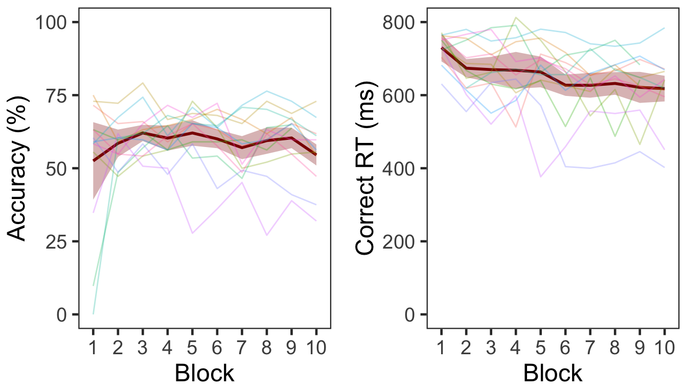
Two participants (6th & 7th) did not make responses in all or most of trials in Block 1. Participants made faster correct responses while maintaining a similar level of accuracy over time. Overall accuracy was 58.64% (s.d. = 8.25).
2 Item Repetition Phase
The same three-phase procedure as in Experiments 1 and 2 was conducted on Day 2. In the item repetition phase, half of the pseudowords learned on Day 1 were repeated eight times, resulting in 192 trials. In each trial, participants made a preference judgment (like/dislike).
P1 <- read.csv("data/data_FamSM_Exp3B_Word_REP.csv", header = T)
P1$Pref <- ifelse(P1$Resp==1,1,0)
glimpse(P1, width=70)
## Observations: 2,496
## Variables: 8
## $ SID     <int> 1, 1, 1, 1, 1, 1, 1, 1, 1, 1, 1, 1, 1, 1, 1, 1, 1, …
## $ RepTime <int> 1, 1, 1, 1, 1, 1, 1, 1, 1, 1, 1, 1, 1, 1, 1, 1, 1, …
## $ Trial   <int> 1, 2, 3, 4, 5, 6, 7, 8, 9, 10, 11, 12, 13, 14, 15, …
## $ Resp    <int> 2, 2, 2, 2, 2, 2, 2, 2, 2, 1, 2, 2, 2, 2, 2, 2, 1, …
## $ Corr    <int> 1, 1, 1, 1, 1, 1, 1, 1, 1, 1, 1, 1, 1, 1, 1, 1, 1, …
## $ RT      <dbl> 1226.19, 752.28, 673.00, 745.71, 634.42, 667.20, 69…
## $ ImgName <fct> nonwin2_8.png, nonwin2_4.png, nonwex4.png, nonwex2_…
## $ Pref    <dbl> 0, 0, 0, 0, 0, 0, 0, 0, 0, 1, 0, 0, 0, 0, 0, 0, 1, …
# 1. SID: participant ID
# 2. RepTime: number of repetition, 1~8
# 3. Trial: 1~24
# 4. Resp: preference judgment, 1 = like, 2 = dislike, 3 = no response
# 5. Corr: correctness, 1 = response, 0 = no response
# 6. RT: reaction times in ms.
# 7. ImgName: name of stimuli
# 8. Pref: preference, 0 = dislike (treating no response as 'dislike'), 1 = like

table(P1$SID)
##
##   1   2   3   4   5   6   7   8   9  10  11  12  13
## 192 192 192 192 192 192 192 192 192 192 192 192 192
Participants did not make responses in 3.04% of trials.
2.1 Preference
The preference score averaged across participants was 47.44%. In the following plot, the red point and error bars represent the mean and 95% bootstrapped CIs.
P1slong <- P1 %>% group_by(SID) %>%
  summarise(Preference = mean(Pref)) %>%
  ungroup()

ggplot(data=P1slong, aes(x=1, y=Preference)) +
  geom_violin(width = 1, trim = TRUE) +
  ggbeeswarm::geom_quasirandom(dodge.width = 0.7, color = "blue", size = 3, alpha = 0.2,
                               show.legend = FALSE) +
  stat_summary(fun.data = "mean_cl_boot", color = "darkred", size = 1) +
  coord_flip(ylim = c(0, 1), clip = "on") +
  labs(y = "Preference Judgment (0 = dislike, 1 = like)") +
  theme_bw(base_size = 18) +
  theme(panel.grid.major = element_blank(),
        panel.grid.minor = element_blank(),
        axis.title.y = element_blank(),
        axis.ticks.y = element_blank(),
        axis.text.y = element_blank(),
        aspect.ratio = .3)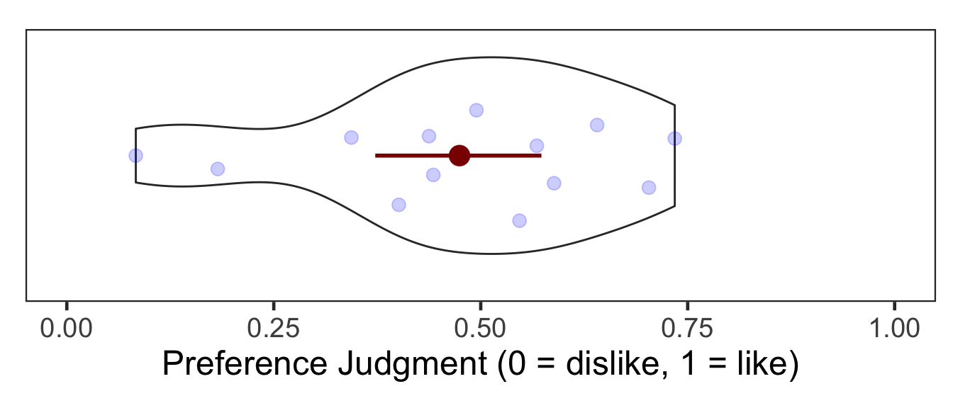
3 Item-Source Association Phase
Participants learned 48 pseudoword-location (a quadrant on the screen) associations. They were instructed to pay attention to the location of each pseudoword while making a preference judgment. All pseudowords shown on Day 1 were presented once in one of four quadrants. Item repetition was the single within-participant independent variable. Half of the pseudowords had been repeated in the first phase (repeated) while the other half had not (unrepeated).
P2 <- read.csv("data/data_FamSM_Exp3B_Word_SRC.csv", header = T)
P2$Repetition = factor(P2$Repetition, levels=c(1,2), labels=c("Repetition","No Repetition"))
P2$Pref <- ifelse(P2$Resp==1,1,0)

glimpse(P2, width=70)
## Observations: 624
## Variables: 9
## $ SID        <int> 1, 1, 1, 1, 1, 1, 1, 1, 1, 1, 1, 1, 1, 1, 1, 1, …
## $ Trial      <int> 1, 2, 3, 4, 5, 6, 7, 8, 9, 10, 11, 12, 13, 14, 1…
## $ Repetition <fct> Repetition, No Repetition, Repetition, No Repeti…
## $ Loc        <int> 4, 4, 2, 1, 2, 2, 4, 2, 1, 3, 2, 1, 4, 1, 3, 2, …
## $ Resp       <int> 1, 1, 1, 1, 1, 1, 1, 2, 1, 1, 2, 1, 1, 1, 1, 1, …
## $ Corr       <int> 1, 1, 1, 1, 1, 1, 1, 1, 1, 1, 1, 1, 1, 1, 1, 1, …
## $ RT         <dbl> 1664.67, 1228.73, 1697.13, 1421.39, 1449.71, 122…
## $ ImgName    <fct> nonwex6.png, nonwex2_4.png, nonwex3.png, nonwin2…
## $ Pref       <dbl> 1, 1, 1, 1, 1, 1, 1, 0, 1, 1, 0, 1, 1, 1, 1, 1, …
# 1. SID: participant ID
# 2. Trial: 1~48
# 3. Repetition: 1 = repetition, 2 = no repetition
# 4. Loc: location (source) of memory item; quadrants, 1~4
# 5. Resp: preference judgment, 1 = like, 2 = dislike, 3 = no response
# 6. Corr: correctness, 1=response, 0 = no response
# 7. RT: reaction times in ms.
# 8. ImgName: name of stimuli
# 9. Pref: preference, 0 = dislike (treating no response as 'dislike'), 1 = like

table(P2$Repetition, P2$SID)
##
##                  1  2  3  4  5  6  7  8  9 10 11 12 13
##   Repetition    24 24 24 24 24 24 24 24 24 24 24 24 24
##   No Repetition 24 24 24 24 24 24 24 24 24 24 24 24 24
Participants did not make responses in 2.72% of trials.
3.1 Preference
We calculated the mean and s.d. of individual participants’ preference score for each condition. As in Experiment 2, preference for pseudowords increased after repetition. In the following plot, red points and error bars represent the means and 95% CIs.
# phase 1, subject-level, long-format
P2slong <- P2 %>% group_by(SID, Repetition) %>%
  summarise(Preference = mean(Pref)) %>%
  ungroup()

# summary table
P2g <- P2slong %>% group_by(Repetition) %>%
  summarise(M = mean(Preference), SD = sd(Preference)) %>%
  ungroup()
P2g %>% kable()| Repetition | M | SD |
|---|---|---|
| Repetition | 0.5448718 | 0.2450089 |
| No Repetition | 0.4038462 | 0.2407938 |
# group level, needed for printing & geom_pointrange
# Rmisc must be called indirectly due to incompatibility between plyr and dplyr.
P2g$ci <- Rmisc::summarySEwithin(data = P2slong, measurevar = "Preference", idvar = "SID", withinvars = "Repetition")$ci
P2g$Preference <- P2g$M

ggplot(P2slong, aes(x=Repetition, y=Preference, fill=Repetition)) +
  geom_violin(width = 0.5, trim=TRUE) +
  ggbeeswarm::geom_quasirandom(color = "blue", size = 3, alpha = 0.2, width = 0.2, show.legend = FALSE) +
  geom_pointrange(P2g, inherit.aes=FALSE,
                  mapping=aes(x = Repetition, y=Preference,
                              ymin = Preference - ci, ymax = Preference + ci),
                  colour="darkred", size = 1) +
  coord_cartesian(ylim = c(0, 1), clip = "on") +
  labs(x = "Item Repetition",
       y = "Preference Judgment \n (0 = dislike, 1 = like)") +
  scale_fill_manual(values=c("#E69F00", "#56B4E9"),
                    labels=c("Repeated", "Unrepeated")) +
  theme_bw(base_size = 18) +
  theme(panel.grid.major = element_blank(),
        panel.grid.minor = element_blank(),
legend.position = "none") 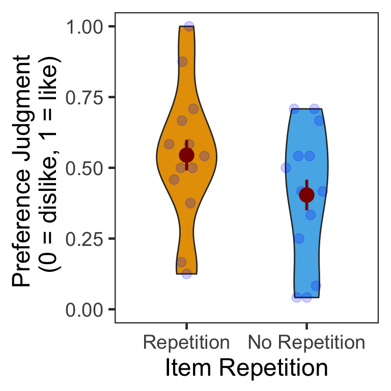
3.1.1 ANOVA
Mean preference scores were submitted to a one-way repeated measures ANOVA. Participants made significantly more ‘Like’ responses to repeated than unrepeated pseudowords (familiarity benefit).
p2.aov <- aov_ez(id = "SID", dv = "Preference", data = P2slong, within = "Repetition")
anova(p2.aov, es = "pes") %>% kable(digits = 4)| num Df | den Df | MSE | F | pes | Pr(>F) | |
|---|---|---|---|---|---|---|
| Repetition | 1 | 12 | 0.008 | 16.0886 | 0.5728 | 0.0017 |
4 Source Memory Test Phase
In each trial, participants first indicated in which quadrant a given pseudoword appeared during the item-source association phase. Participants then rated how confident they were about their memory judgment.
P3 <- read.csv("data/data_FamSM_Exp3B_Word_TST.csv", header = T)
P3$Repetition = factor(P3$Repetition, levels=c(1,2), labels=c("Repeated","Unrepeated"))

glimpse(P3, width=70)
## Observations: 624
## Variables: 9
## $ SID        <int> 1, 1, 1, 1, 1, 1, 1, 1, 1, 1, 1, 1, 1, 1, 1, 1, …
## $ Trial      <int> 1, 2, 3, 4, 5, 6, 7, 8, 9, 10, 11, 12, 13, 14, 1…
## $ Repetition <fct> Unrepeated, Repeated, Unrepeated, Unrepeated, Un…
## $ AscLoc     <int> 2, 4, 4, 1, 3, 4, 4, 1, 2, 1, 2, 4, 4, 4, 3, 1, …
## $ ScrResp    <int> 2, 1, 4, 1, 3, 4, 4, 1, 2, 1, 1, 1, 4, 4, 4, 3, …
## $ Corr       <int> 1, 0, 1, 1, 1, 1, 1, 1, 1, 1, 0, 0, 1, 1, 0, 0, …
## $ RT         <dbl> 2144.57, 6669.51, 1793.32, 1672.23, 1580.44, 132…
## $ Confident  <int> 4, 1, 4, 4, 4, 4, 4, 2, 1, 4, 1, 1, 4, 4, 1, 1, …
## $ ImgName    <fct> nonwex2_2.png, nonwin2.png, nonwex12.png, nonwex…
# 1. SID: participant ID
# 2. Trial: 1~48
# 3. Repetition: 1 = repetition, 2 = no repetition
# 4. AscLoc: location (source) in which the item was presented in Phase 2; quadrants, 1~4
# 5. SrcResp: source response; quadrants, 1~4
# 6. Corr: correctness, 1=correct ,2=incorrect & no response
# 7. RT: reaction times in ms.
# 8. Confident: confidence rating, 1~4
# 9. ImgName: name of stimuli

table(P3$Repetition, P3$SID)
##
##               1  2  3  4  5  6  7  8  9 10 11 12 13
##   Repeated   24 24 24 24 24 24 24 24 24 24 24 24 24
##   Unrepeated 24 24 24 24 24 24 24 24 24 24 24 24 24
4.1 Accuracy
We calculated the mean and s.d. of individual participants’ mean percentage accuracy. Source memory accuracy was greater in the unrepeated than repeated condition (novelty benefit). In the following plot, red points and error bars represent the means and 95% within-participants CIs.
# phase 3, subject-level, long-format
P3ACCslong <- P3 %>% group_by(SID, Repetition) %>%
  summarise(Accuracy = mean(Corr)*100) %>%
  ungroup()

# summary table
P3ACCg <- P3ACCslong %>% group_by(Repetition) %>%
  summarise(M = mean(Accuracy), SD = sd(Accuracy)) %>%
  ungroup()
P3ACCg %>% kable()| Repetition | M | SD |
|---|---|---|
| Repeated | 40.38462 | 14.27092 |
| Unrepeated | 49.35897 | 17.82812 |
# wide format, needed for geom_segments.
P3ACCswide <- P3ACCslong %>% spread(key = Repetition, value = Accuracy)

# group level, needed for printing & geom_pointrange
# Rmisc must be called indirectly due to incompatibility between plyr and dplyr.
P3ACCg$ci <- Rmisc::summarySEwithin(data = P3ACCslong, measurevar = "Accuracy", idvar = "SID", withinvars = "Repetition")$ci
P3ACCg$Accuracy <- P3ACCg$M

ggplot(data=P3ACCslong, aes(x=Repetition, y=Accuracy, fill=Repetition)) +
  geom_violin(width = 0.5, trim=TRUE) +
  geom_point(position=position_dodge(0.5), color="gray80", size=1.8, show.legend = FALSE) +
  geom_segment(data=P3ACCswide, inherit.aes = FALSE,
               aes(x=1, y=P3ACCswide$Repeated, xend=2, yend=P3ACCswide$Unrepeated), color="gray80") +
  geom_pointrange(data=P3ACCg,
                  aes(x = Repetition, ymin = Accuracy-ci, ymax = Accuracy+ci, group = Repetition),
                  position = position_dodge(0.5), color = "darkred", size = 1, show.legend = FALSE) +
  scale_fill_manual(values=c("#E69F00", "#56B4E9"),
                    labels=c("Repeated", "Unrepeated")) +
  labs(x = "Item Repetition",
       y = "Source Memory Accuracy (%)") +
  coord_cartesian(ylim = c(0, 100), clip = "on") +
  theme_bw(base_size = 18) +
  theme(panel.grid.major = element_blank(),
        panel.grid.minor = element_blank(),
        legend.position = "none")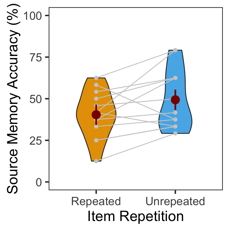
4.1.1 ANOVA
Mean percentage accuracy was submitted to a one-way repeated measures ANOVA.
ci95 <- P3ACCswide %>%
  mutate(Diff = Unrepeated - Repeated) %>%
  summarise(lower = mean(Diff) - qt(0.975,df=n()-1)*sd(Diff)/sqrt(n()),
            upper = mean(Diff) + qt(0.975,df=n()-1)*sd(Diff)/sqrt(n()))

p3.corr.aov <- aov_ez(id = "SID", dv = "Accuracy", data = P3ACCslong, within = "Repetition")
anova(p3.corr.aov, es = "pes") %>% kable(digits = 4)| num Df | den Df | MSE | F | pes | Pr(>F) | |
|---|---|---|---|---|---|---|
| Repetition | 1 | 12 | 102.4973 | 5.1075 | 0.2986 | 0.0432 |
Source memory accuracy was higher for unrepeated than repeated pseudowords. The 95% CI of difference between the means was [0.32, 17.63].
4.1.2 GLMM
To supplement conventional ANOVAs, we tested generalized linear mixed models (GLMM) on source memory accuracy. This mixed modeling approach with a binomial link function is expected to properly handle binary data such as source memory responses (i.e., correct or not; Jaeger, 2008).
The full model (full1) was built with a fixed effect (item repetition). The model was maximal in that it included both by-participant and by-item random intercepts, and by-participant random slopes for item repetition (Barr, Levy, Scheepers, & Tily, 2013). In case the maximal model does not converge successfully, we built another model (full2) with the maximal random structure but with the correlations among the random terms removed (Singmann, 2018).
To fit the models, we used the mixed() of the afex package (Singmann, Bolker, & Westfall, 2017) which was built on the lmer() of the lme4 package (Bates, Maechler, Bolker, & Walker, 2015). The mixed() assessed the statistical significance of fixed effects by comparing a model with the effect in question against its nested model which lacked the effect in question. P-values of the effects were obtained by likelihood ratio tests (LRT).
(nc <- detectCores())
cl <- makeCluster(rep("localhost", nc))

full1 <- mixed(Corr ~ Repetition + (Repetition|SID) + (1|ImgName),
               P3, method = "LRT", cl = cl,
               family=binomial(link="logit"),
               control = glmerControl(optCtrl = list(maxfun = 1e6)))
full2 <- mixed(Corr ~ Repetition + (Repetition||SID) + (1|ImgName),
               P3, method = "LRT", cl = cl,
               family=binomial(link="logit"),
               control = glmerControl(optCtrl = list(maxfun = 1e6)), expand_re = TRUE)

stopCluster(cl)
The table below shows the LRT results of the models full1 and full2 side by side.
full.compare <- cbind(afex::nice(full1), afex::nice(full2)[,-c(1,2)])
colnames(full.compare)[c(3,4,5,6)] <- c("full1 Chisq", "p","full2 Chisq", "p")
full.compare %>% kable()| Effect | df | full1 Chisq | p | full2 Chisq | p |
|---|---|---|---|---|---|
| Repetition | 1 | 4.37 * | .04 | 4.68 * | .03 |
The p-values from the two models were highly similar to each other. Item repetition impaired source memory for pseudowords that were familiarized on the previous day.
4.2 Confidence
The following table presents the mean and s.d. of individual participants’ confidence ratings in each condition. There was no difference between the repeated vs. unrepeated conditions.
P3CFslong <- P3 %>% group_by(SID, Repetition) %>%
  summarise(Confidence = mean(Confident)) %>%
  ungroup()

P3CFg <- P3CFslong %>% group_by(Repetition) %>%
  summarise(M = mean(Confidence), SD = sd(Confidence)) %>%
  ungroup()
P3CFg %>% kable()| Repetition | M | SD |
|---|---|---|
| Repeated | 2.490385 | 0.5254390 |
| Unrepeated | 2.493590 | 0.5346355 |
# wide format, needed for geom_segments.
P3CFswide <- P3CFslong %>% spread(key = Repetition, value = Confidence)

# group level, needed for printing & geom_pointrange
# Rmisc must be called indirectly due to incompatibility between plyr and dplyr.
P3CFg$ci <- Rmisc::summarySEwithin(data = P3CFslong, measurevar = "Confidence", idvar = "SID", withinvars = "Repetition")$ci
P3CFg$Confidence <- P3CFg$M

ggplot(data=P3CFslong, aes(x=Repetition, y=Confidence, fill=Repetition)) +
  geom_violin(width = 0.5, trim=TRUE) +
  geom_point(position=position_dodge(0.5), color="gray80", size=1.8, show.legend = FALSE) +
  geom_segment(data=P3CFswide, inherit.aes = FALSE,
               aes(x=1, y=P3CFswide$Repeated, xend=2, yend=P3CFswide$Unrepeated), color="gray80") +
  geom_pointrange(data=P3CFg,
                  aes(x = Repetition, ymin = Confidence-ci, ymax = Confidence+ci, group = Repetition),
                  position = position_dodge(0.5), color = "darkred", size = 1, show.legend = FALSE) +
  scale_fill_manual(values=c("#E69F00", "#56B4E9"),
                    labels=c("Repeated", "Unrepeated")) +
  labs(x = "Item Repetition",
       y = "Source Memory Confidence") +
  coord_cartesian(ylim = c(1, 4), clip = "on") +
  theme_bw(base_size = 18) +
  theme(panel.grid.major = element_blank(),
        panel.grid.minor = element_blank(),
        legend.position = "none")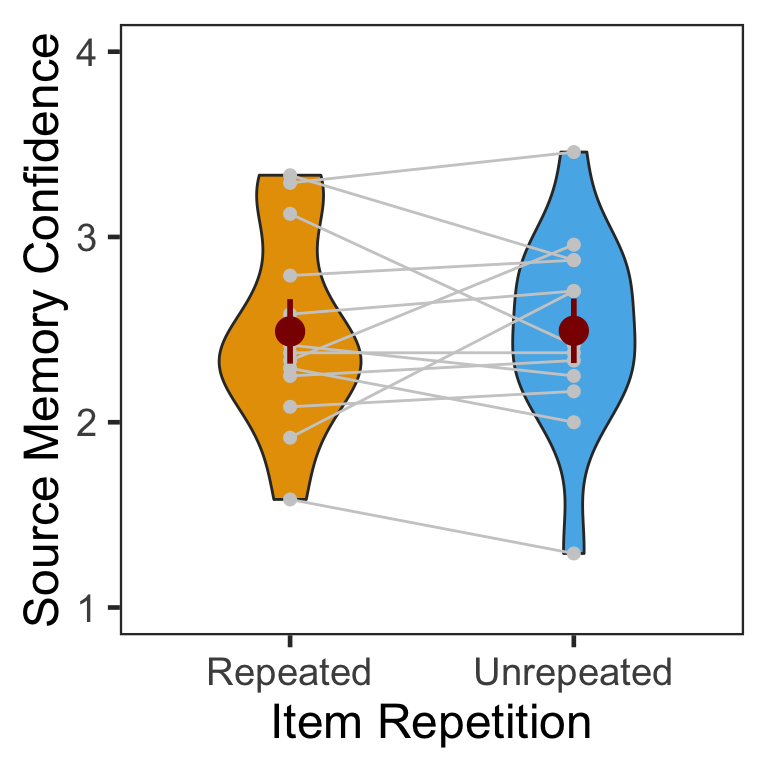
4.2.1 ANOVA
Mean confidence ratings were submitted to a one-way repeated measures ANOVA.
ci95 <- P3CFswide %>%
  mutate(Diff = Unrepeated - Repeated) %>%
  summarise(lower = mean(Diff) - qt(0.975,df=n()-1)*sd(Diff)/sqrt(n()),
            upper = mean(Diff) + qt(0.975,df=n()-1)*sd(Diff)/sqrt(n()))

p3.conf.aov <- aov_ez(id = "SID", dv = "Confidence", data = P3CFslong, within = "Repetition")
anova(p3.conf.aov, es = "pes") %>% kable(digits = 4)| num Df | den Df | MSE | F | pes | Pr(>F) | |
|---|---|---|---|---|---|---|
| Repetition | 1 | 12 | 0.083 | 8e-04 | 1e-04 | 0.9778 |
The difference between conditions was not significant. The 95% CI of difference between the means was [-0.24, 0.25].
4.2.2 CLMM
The responses from a Likert-type scale are ordinal. Especially for the rating items with numerical response formats containing four or fewer categories, it is recommended to use categorical data analysis approaches, rather than treating the responses as continuous data (Harpe, 2015).
Here we employed the cumulative link mixed modeling using the clmm() of the package ordinal (Christensen, submitted). The model specification of fixed and random effects was the same as the mixed() above.
P3R <- P3
P3R$Confident = factor(P3R$Confident, ordered = TRUE)
P3R$SID = factor(P3R$SID)

cm.full <- clmm(Confident ~ Repetition + (Repetition|SID) + (1|ImgName), data=P3R)
cm.red1 <- clmm(Confident ~ 1 + (Repetition|SID) + (1|ImgName), data=P3R)
To determine the significance of the fixed effect, the LRT compared the full model (cm.full) with its nested model (cm.red1) without the effect of interest. The next table shows that the effect of item repetition was not significant.
cm.comp <- anova(cm.full, cm.red1)
data.frame(Effect = "Repetition", df = 1, Chisq = cm.comp$LR.stat[2], p = cm.comp$`Pr(>Chisq)`[2]) %>% kable()| Effect | df | Chisq | p |
|---|---|---|---|
| Repetition | 1 | 0.0101446 | 0.9197723 |
Below is the plot of estimated marginal means, which were extracted from the fitted CLMM. There was little difference between conditions in the distribution of ratings.
pacman::p_load(RVAideMemoire)
temp <- emmeans(cm.full,~Repetition|cut,mode="linear.predictor")
temp <- rating.emmeans(temp)

colnames(temp)[1] <- "Condition"

ggplot(data = temp, aes(x = Rating, y = Prob, group = Condition)) +
  geom_line(aes(color = Condition), size = 1.2) +
  geom_point(aes(shape = Condition, color = Condition),
             size = 4, fill = "white", stroke = 1.2) +
  scale_color_manual(values=c("#E69F00", "#E69F00")) +
  scale_shape_manual(name="Condition", values=c(21,24)) +
  labs(y = "Response Probability", x = "Rating") +
  expand_limits(y=0) +
  scale_y_continuous(limits = c(0, 0.5)) +
  scale_x_discrete(labels = c("1" = "1(Guessed)","4"="4(Sure)")) +
  theme_minimal() +
  theme(text = element_text(size=18))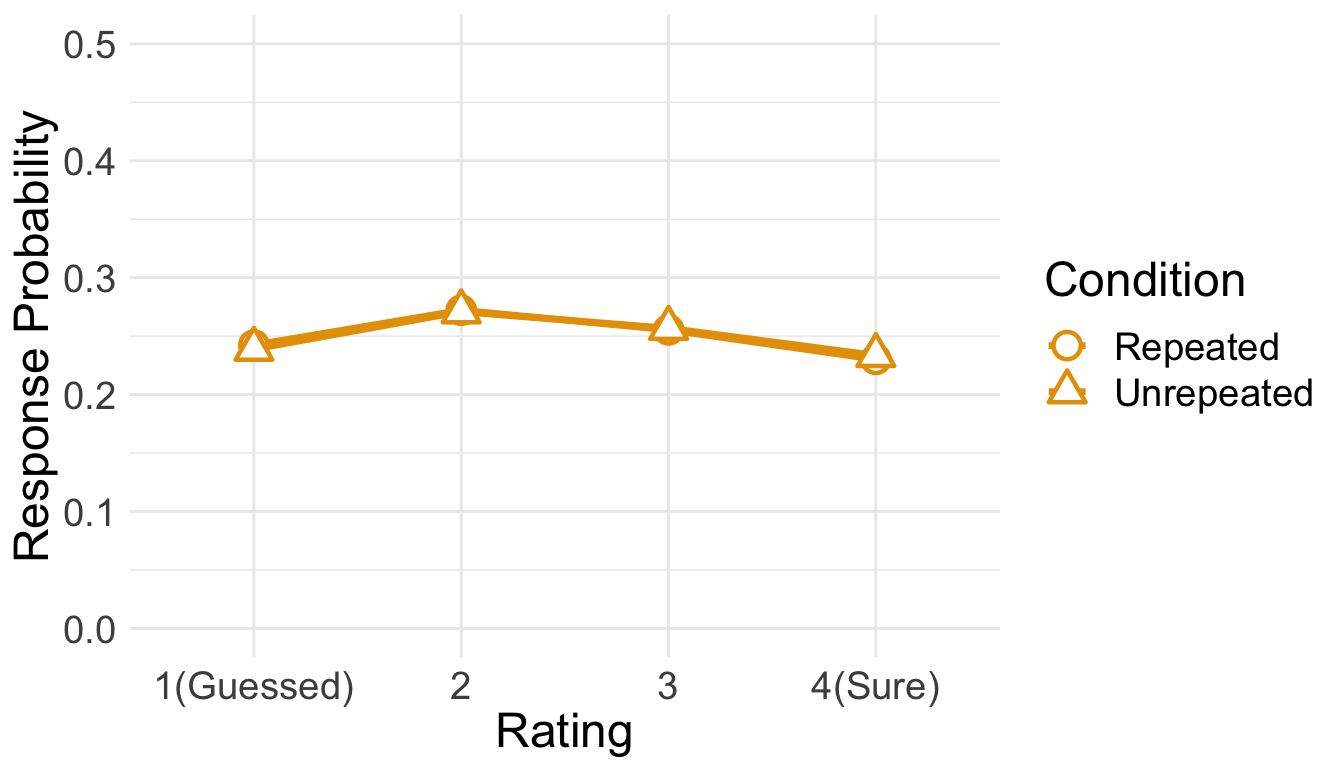
4.3 RT
Only RTs from correct trials were analyzed. Before analysis, we first removed RTs either shorter than 200ms or longer than 10s. Then, from the RT distribution of each condition, RTs beyond 3 s.d. from the mean were additionally removed.
cP3 <- P3 %>% filter(Corr==1)

sP3 <- cP3 %>% filter(RT > 200 & RT < 10000) %>%
  group_by(SID) %>%
  nest() %>%
  mutate(lbound = map(data, ~mean(.$RT)-3*sd(.$RT)),
         ubound = map(data, ~mean(.$RT)+3*sd(.$RT))) %>%
  unnest(lbound, ubound) %>%
  unnest(data) %>%
  ungroup() %>%
  mutate(Outlier = (RT < lbound)|(RT > ubound)) %>%
  filter(Outlier == FALSE) %>%
  select(SID, Repetition, RT, ImgName)

100 - 100*nrow(sP3)/nrow(cP3)
## [1] 2.857143
This trimming procedure removed 2.86% of correct trials.
Since the overall source memory accuracy was not high, only small numbers of correct trials were available after trimming. The following table summarizes the numbers of RTs submitted to subsequent analyses. No participant had more than 20 trials per condition.
sP3 %>% group_by(SID, Repetition) %>%
  summarise(NumTrial = length(RT)) %>%
  ungroup %>%
  group_by(Repetition) %>%
  summarise(Avg = mean(NumTrial),
            Med = median(NumTrial),
            Min = min(NumTrial),
            Max = max(NumTrial)) %>%
  ungroup %>%
kable()| Repetition | Avg | Med | Min | Max |
|---|---|---|---|---|
| Repeated | 9.538462 | 10 | 3 | 15 |
| Unrepeated | 11.384615 | 10 | 6 | 19 |
den1 <- ggplot(cP3, aes(x=RT)) +
  geom_density() +
  theme_bw(base_size = 18) +
  theme(panel.grid.major = element_blank(),
        panel.grid.minor = element_blank(),
        axis.text.y = element_blank(),
        axis.ticks.y = element_blank())
den2 <- ggplot(sP3, aes(x=RT)) +
  geom_density() +
  theme_bw(base_size = 18) +
  labs(x = "Trimmed RT") +
  theme(panel.grid.major = element_blank(),
        panel.grid.minor = element_blank(),
        axis.text.y = element_blank(),
        axis.ticks.y = element_blank())
den1 + den2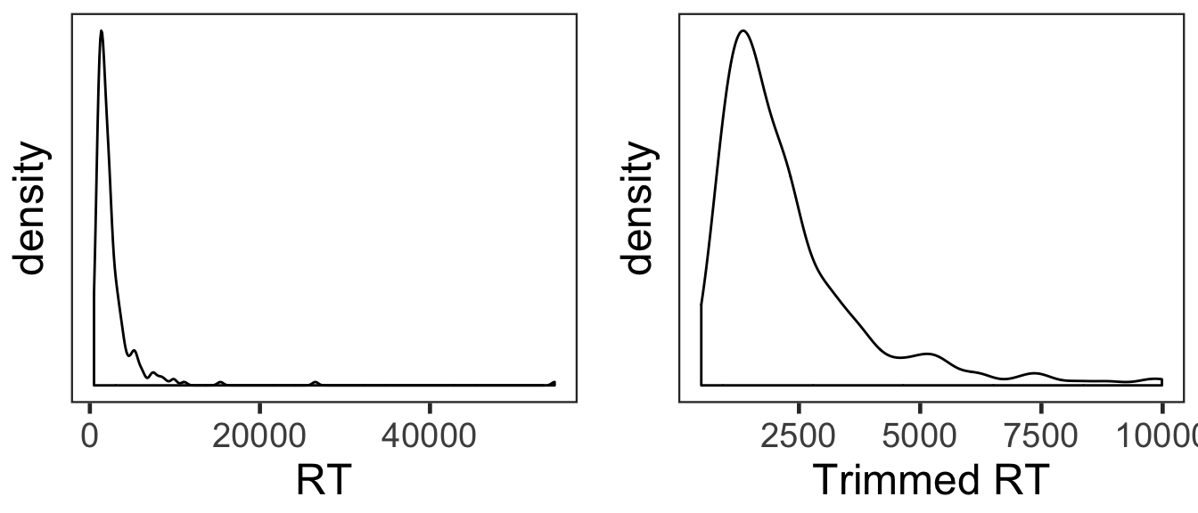
The overall RT distribution was highly skewed even after trimming. Given limited numbers of RTs and its skewed distribution, any results from the current RT analyses should be interpreted with caution and preferably corroborated with other measures.
We calculated the mean and s.d. of individual participants’ mean RTs. The overall pattern of RTs was consistent with that of source memory accuracy and confidence ratings. Participants made slightly faster responses in the repeated than unrepeated condition.
P3RTslong <- sP3 %>% group_by(SID, Repetition) %>%
  summarise(RT = mean(RT)) %>%
  ungroup()

P3RTg <- P3RTslong %>% group_by(Repetition) %>%
  summarise(M = mean(RT), SD = sd(RT)) %>%
  ungroup()
P3RTg %>% kable()| Repetition | M | SD |
|---|---|---|
| Repeated | 2239.234 | 342.7272 |
| Unrepeated | 2316.788 | 1227.0245 |
# wide format, needed for geom_segments.
P3RTswide <- P3RTslong %>% spread(key = Repetition, value = RT)

# group level, needed for printing & geom_pointrange
# Rmisc must be called indirectly due to incompatibility between plyr and dplyr.
P3RTg$ci <- Rmisc::summarySEwithin(data = P3RTslong, measurevar = "RT", idvar = "SID", withinvars = "Repetition")$ci
P3RTg$RT <- P3RTg$M

ggplot(data=P3RTslong, aes(x=Repetition, y=RT, fill=Repetition)) +
  geom_violin(width = 0.5, trim=TRUE) +
  geom_point(position=position_dodge(0.5), color="gray80", size=1.8, show.legend = FALSE) +
  geom_segment(data=P3RTswide, inherit.aes = FALSE,
               aes(x=1, y=P3RTswide$Repeated, xend=2, yend=P3RTswide$Unrepeated), color="gray80") +
  geom_pointrange(data=P3RTg,
                  aes(x = Repetition, ymin = RT-ci, ymax = RT+ci, group = Repetition),
                  position = position_dodge(0.5), color = "darkred", size = 1, show.legend = FALSE) +
  scale_fill_manual(values=c("#E69F00", "#56B4E9"),
                    labels=c("Repeated", "Unrepeated")) +
  labs(x = "Item Repetition",
       y = "Response Times (ms)") +
  coord_cartesian(ylim = c(0, 6000), clip = "on") +
  theme_bw(base_size = 18) +
  theme(panel.grid.major = element_blank(),
        panel.grid.minor = element_blank(),
        legend.position = "none")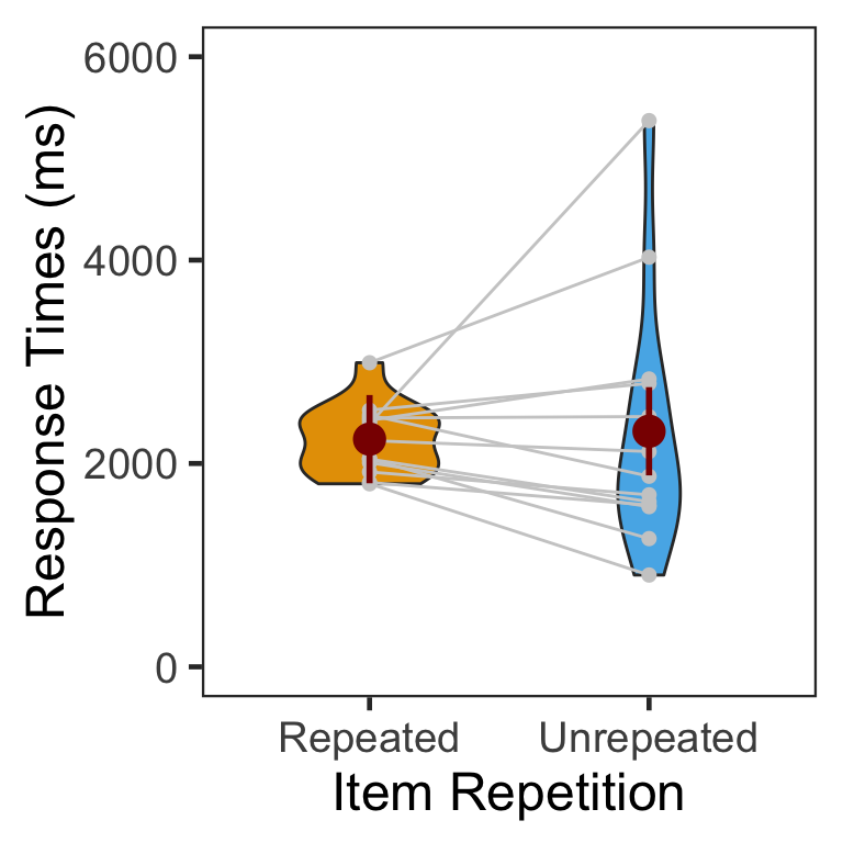
4.3.1 ANOVA
Individuals’ mean RTs were submitted to a one-way repeated measures ANOVA with item repetition as a within-participant factor. The RT difference between conditions was not significant.
p3.rt.aov <- aov_ez(id = "SID", dv = "RT", data = sP3, within = "Repetition")
anova(p3.rt.aov, es = "pes") %>% kable(digits = 4)| num Df | den Df | MSE | F | pes | Pr(>F) | |
|---|---|---|---|---|---|---|
| Repetition | 1 | 12 | 515619.4 | 0.0758 | 0.0063 | 0.7877 |
5 Session Info
sessionInfo()
## R version 3.5.3 (2019-03-11)
## Platform: x86_64-apple-darwin15.6.0 (64-bit)
## Running under: macOS Mojave 10.14.4
##
## Matrix products: default
## BLAS: /Library/Frameworks/R.framework/Versions/3.5/Resources/lib/libRblas.0.dylib
## LAPACK: /Library/Frameworks/R.framework/Versions/3.5/Resources/lib/libRlapack.dylib
##
## locale:
## [1] en_US.UTF-8/en_US.UTF-8/en_US.UTF-8/C/en_US.UTF-8/en_US.UTF-8
##
## attached base packages:
## [1] parallel  stats     graphics  grDevices utils     datasets  methods
## [8] base
##
## other attached packages:
##  [1] klippy_0.0.0.9500    patchwork_0.0.1      RVAideMemoire_0.9-73
##  [4] ggbeeswarm_0.6.0     ordinal_2019.3-9     emmeans_1.3.3
##  [7] afex_0.23-0          lme4_1.1-21          Matrix_1.2-17
## [10] car_3.0-2            carData_3.0-2        knitr_1.22
## [13] forcats_0.4.0        stringr_1.4.0        dplyr_0.8.0.1
## [16] purrr_0.3.2          readr_1.3.1          tidyr_0.8.3
## [19] tibble_2.1.1         ggplot2_3.1.0        tidyverse_1.2.1
## [22] Rmisc_1.5            plyr_1.8.4           lattice_0.20-38
## [25] pacman_0.5.1
##
## loaded via a namespace (and not attached):
##  [1] TH.data_1.0-10      minqa_1.2.4         colorspace_1.4-1
##  [4] rio_0.5.16          htmlTable_1.13.1    estimability_1.3
##  [7] base64enc_0.1-3     rstudioapi_0.10     fansi_0.4.0
## [10] mvtnorm_1.0-10      lubridate_1.7.4     xml2_1.2.0
## [13] codetools_0.2-16    splines_3.5.3       Formula_1.2-3
## [16] jsonlite_1.6        nloptr_1.2.1        broom_0.5.1
## [19] cluster_2.0.7-1     compiler_3.5.3      httr_1.4.0
## [22] backports_1.1.3     assertthat_0.2.1    lazyeval_0.2.2
## [25] cli_1.1.0           acepack_1.4.1       htmltools_0.3.6
## [28] tools_3.5.3         lmerTest_3.1-0      coda_0.19-2
## [31] gtable_0.3.0        glue_1.3.1          reshape2_1.4.3
## [34] Rcpp_1.0.1          cellranger_1.1.0    nlme_3.1-137
## [37] xfun_0.5            openxlsx_4.1.0      rvest_0.3.2
## [40] MASS_7.3-51.3       zoo_1.8-5           scales_1.0.0
## [43] hms_0.4.2           sandwich_2.5-0      RColorBrewer_1.1-2
## [46] yaml_2.2.0          curl_3.3            gridExtra_2.3
## [49] rpart_4.1-13        latticeExtra_0.6-28 stringi_1.4.3
## [52] highr_0.8           ucminf_1.1-4        checkmate_1.9.1
## [55] boot_1.3-20         zip_2.0.1           rlang_0.3.3
## [58] pkgconfig_2.0.2     evaluate_0.13       htmlwidgets_1.3
## [61] labeling_0.3        tidyselect_0.2.5    magrittr_1.5
## [64] R6_2.4.0            generics_0.0.2      Hmisc_4.2-0
## [67] multcomp_1.4-10     pillar_1.3.1        haven_2.1.0
## [70] foreign_0.8-71      withr_2.1.2         survival_2.44-1
## [73] abind_1.4-5         nnet_7.3-12         modelr_0.1.4
## [76] crayon_1.3.4        utf8_1.1.4          rmarkdown_1.12
## [79] grid_3.5.3          readxl_1.3.1        data.table_1.12.0
## [82] digest_0.6.18       xtable_1.8-3        numDeriv_2016.8-1
## [85] munsell_0.5.0       beeswarm_0.2.3      vipor_0.4.5